A logic-algebraic tool for reasoning with Knowledge-Based SystemsThis work was partially supported by TIN2013-41086-P project (Spanish Ministry of Economy and Competitiveness), co-financed with FEDER funds.

José A. Alonso-Jiménez¹, Gonzalo A. Aranda-Corral², Joaquín Borrego-Díaz¹, M. Magdalena Fernández-Lebrón³, M. José Hidalgo-Doblado¹ Address: ¹Departamento de Ciencias de la Computación e Inteligencia Artificial, E.T.S. Ingeniería Informática, Universidad de Sevilla, Avda. Reina Mercedes s.n. 41012-Sevilla, Spain
² Department of Information Technology, Universidad de Huelva Crta. Palos de La Frontera s/n. 21819 Palos de La Frontera. Spain
³Departamento de Matemática Aplicada I, E.T.S. Ingeniería Informática, Universidad de Sevilla, Avda. Reina Mercedes s.n. 41012-Sevilla, Spain

Abstract

A detailed exposition of foundations of a logic-algebraic model for reasoning with knowledge bases specified by propositional (Boolean) logic is presented. The model is conceived from the logical translation of usual derivatives on polynomials (on residue rings) which is used to design a new inference rule of algebro-geometric inspiration. Soundness and (refutational) completeness of the rule are proved. Some applications of the tools introduced in the paper are shown.

Keywords:

Polynomial Semantics , Symbolic Computing , Automated Deduction , Knowledge-Based Systems

1 Introduction

Algebraic models for logic have been revealed as a useful tool for knowledge representation and mechanized reasoning. The relationship between certain algebraic structures and Computational Logic provides methods and tools for building, compiling and reasoning with Knowledge-Based Systems (KBS) (see e.g. [1] for an introduction). This relationship also provides mathematical foundations for a number of Knowledge Representation and Reasoning (KRR) methods and algorithms, encompassing applications since the pioneer works for classical bivalued logic [2, 3] to extensions for multi-valued logics [4, 5, 6, 7]. The framework has also been extended to other logics for Artificial Intelligence (AI) as the paraconsistent logic [8], and even towards other nonstandard reasoning tasks as the argument-based one (cf. [9]). One of the benefits of the interpretation of logic in polynomial rings is that enables the use of powerful algebraic tools as Gröbner Basis to compile KBS, exploiting this way the use of advanced Computer Algebra Systems in KRR.

Roughly speaking, algebraic models for logic are mainly based on to specify, obtain and exploit solutions for the logical entailment problem and other related ones. Recall that the entailment problem in logic is stated as follows: given a Knowledge Base (KB) $K$ , and a formula $F$ , to decide whether $F$ is a logical consequence from $K$ (denoted by $K\models F$ ), that is, whether every model of $K$ is also model of $F$ .

This paper is focused in to expound with detail an(other) algebraic model for KRR. Whilst aforementioned approaches do not need to design a new calculus (ideal membership translation -through Gröbner Basis- of entailment question is sufficient), the approach presented here consists of to design an inference rule -called independence rule- from an algebraic operation on polynomials¹¹ 1 The part of the paper devoted to this is an extended version of [10].. This rule will allow address a number of other related problems.

Although the independence rule is inspired in Algebra, the idea is intimately related with KRR strategies which are oriented to mitigate the complexity and size of the $KB$ (which may be of large size), with the hope of reducing the computational cost of the deductive process when it is applied into specialized contexts or use cases. Two strategies of this type are interesting for the purposes of the paper and motivate this work.

The first is to facilitate the design of divide-and-conquer strategies to deal with the entailment problem, a natural idea for managing KBs with hundreds of thousands of logical axioms with big size logical language (for example the strategy based on the reasoning with microtheories [11]). In this case the problem of ensuring the completeness of the designed strategy arises, being a critical issue the selection/synthesis of sound sub-KBs. In [12] authors propose a partition-based strategy in order to obtain subtheories. It is based on a syntax level analysis that provides individual partitions where to reason locally, and distributed reasoning needs of methods to propagate information among different partitions.

The second strategy to consider is based on the ad-hoc reduction of KB for particular use cases (distilling the KB for using in context-based reasoning, for example). In [10] authors propose to reduce $K$ to $K^{\prime}$ , where $K\models K^{\prime}$ , and in $K^{\prime}$ only the language of the goal formula $F$ is used (thus it is expected that the size of $K^{\prime}$ to be smaller than the size of $K$ ). Then the entailment problem with respect to $K^{\prime}$ is considered. For this strategy to be successful -valid and complete- $K$ must be a conservative extension of $K^{\prime}$ (or, equivalently, $K^{\prime}$ a conservative retraction of $K$ [10]). A knowledge base $K^{\prime}$ in the language $\mathcal{L}^{\prime}$ is a conservative retraction of $K$ if $K$ is an extension of $K^{\prime}$ such that every $\mathcal{L}^{\prime}$ -fórmula entailed by $K$ is also entailed by $K^{\prime}$ . Then the use of conservative retraction allows to reduce the own KB we need to work, because it suffices to conservatively retracts the original KB to the specialized language of the formula-goal. A key question is how to compute such kind of sub-KBs.

Whilst conservative extensions have been deeply investigated in several fields of Mathematical Logic and Computer Science (because they allow the formalization of several notions concerning refinements and modularity, see e.g. [13, 14, 15]), solutions focused on its dual notion, the conservative retraction, are obstructed by its logical complexity (see e.g. [16]).

Beside the analysis of above strategy, as a secondary motivation of the approach, it is worth to mention the study of relevance in knowledge bases. To analyze, locate and remove redundancies in KB is a way to refine and improve the efficiency of KBS. These type of analysis are important in topics such as probabilistic reasoning, information filtering, etc. (see also [16] for a general overview).

The basic mechanism to obtain conservative retractions consists of eliminating, step by step, the variables that we wish to eliminate from language. Such a mechanism is called variable forgetting. Since the first analysis in cognitive robotics [17], the problem of variable forgetting is a widely studied technique in IA. In particular the forgetting variable technique has been used to update or refine (logical, rule-based, CSP) programs. For example for resolution-based reasoning in specialized contexts (see e.g. [18]), in CSP and optimization [19], for simplification of rules [20] (included Answer Set Programming [21]). As it can be seen from these references, the interest in techniques for forgetting variables is not limited to classical (monotonous) logics. It has also received attention in the field of non-monotonous reasoning (including the computational complexity of the problems). In the (epistemic) modal logics for (multi)agency this technique would be very useful to represent knowledge-based games [22, 23]. In addition, in the reasoning under inconsistency the use of variable forgetting allows to weaken the KB to obtain consistent subKBs (eliminating the variables involved in the inconsistency). This topic, discussed below, is studied as a tool for solving SAT. In this context, providing methods for variable forgetting is a step towards the availability of retraction algorithms for programming paradigms based on logics of different nature.

Taking into account the aforementioned motivations, the aim of this paper is twofold. First, we intend to present a complete and detailed exposition of the foundations of the independence rule (That can be considered a tool for variable forgetting), whose basic ideas were published in [10], since no detailed exposition has been published until now. In fact, we generalize the cited paper by stating the results for any operator that induces a conservative retraction, leading as consequence that our case, the independence rule, is useful to compute the retractions. It is also illustrated how the rule is useful to design methods for solving some questions on KB. In particular the redundancy problem can be handled by the independence rule and Boolean derivatives (an essential tool to design this rule).

The structure of the paper is as follows. Section 2 is devoted to summarize the basics on the algebraic interpretation of propositional logics. In Sect. 3 the notion of forgetting operator is introduced, and we show how conservative retractions can be computed by means of these kind of operators, as well as logical calculus induced by them are sound and (refutationally) complete. Section 4 presents a forgetting operator inspired on the projection of algebraic varieties. The logical translation of the operator is presented as a inference rule in Sect. 5. Boolean derivatives are used for characterizing logical relevance (in the case of sensitive variables) in algebraic terms (in section 6, Prop. 6.3). Some illustrative applications of the tools presented are described in Sect. 7. The paper finishes with a discussion on the results presented in the paper as well as some ideas about future work.

2 Background

Refer to caption — Figure 1: The framework

In this section fundamental relations between propositional logic and polynomials with coefficients in finite fields (in our case, the finite field with two elements, ${\mathbb{F}}_{2}$ ) are summarized. The main idea guiding the algebraic interpretation of logic is to identify a logical formula as a polynomial in such a way that the truth-value function induced by the formula could be understood as a polynomial function on ${\mathbb{F}}_{2}$ .

The diagram showed above (Fig. 1) depicts the relationship between both structures, whose elements will be detailed in the following subsections. The ideal ${\mathbb{I}}_{2}:=\langle x_{1}+x_{1}^{2},\dots,x_{n}+x^{2}_{n}\rangle\subseteq{\mathbb{F}}_{2}[{\bf x}]$ -on which we will talk about later- is used, and the map $proj$ is the natural projection on the quotient ring. The remain elements of the diagram will be detailed bellow.

We assume throughout the paper that the reader is familiar with propositional logic as well as with basic principles on polynomial algebra on positive characteristics.

2.1 Propositional logic and conservative retraction

A propositional language is a finite set $\mathcal{L}=\{p_{1},\dots,p_{n}\}$ of propositional symbols (also called propositional variables). The set of formulas $Form(\mathcal{L})$ is built up from in the usual way, using the standard connectives $\lnot,\land,\lor,\to$ and $\top$ ( $\top$ denotes the constant true, and $\bot$ is $\lnot\top$ ). Given two formulas $F,G$ and $p\in\mathcal{L}$ , we denote $F\{p/G\}$ the formula obtained replacing every occurrence of $p$ in $F$ by the formula $G$ .

An interpretation (or valuation) $v$ is a function $v:\mathcal{L}\to\{0,1\}$ . An interpretation $v$ is a model of $F\in Form(\mathcal{L})$ if it makes $F$ true in the usual classical truth functional way. Analogously, it is said that a $v$ is a model of $K$ ( $v\models K$ ) if $v$ is model of every formula in $K$ . We denote by $Mod(F)$ the set of models of $F$ (resp. $Mod(K)$ for the set of models of $K$ ).

A formula $F$ (or $K$ a KB) is consistent if it exhibits at least one model. It is said that $K$ entails $F$ ( $K\models F$ ) if every model of $K$ is a model of $F$ , that is, $Mod(K)\subseteq Mod(F)$ . Both notions can be naturally generalized to a KB, preserving the same notation. It is said that $K$ and $K^{\prime}$ are equivalent, $K^{\prime}\equiv K$ , if $K\models K^{\prime}$ and $K^{\prime}\models K$ . The same notation will also be used for the equivalence with (and between) formulas.

It is said that $K$ is an extension of $K^{\prime}$ if ${\mathcal{L}}(K^{\prime})\subseteq{\mathcal{L}}(K)$ and

\forall F\in Form({\mathcal{L}}(K^{\prime}))[K^{\prime}\models F\quad\Longrightarrow\quad K\models F]

$K$ is a conservative extension of $K^{\prime}$ (or $K^{\prime}$ is a conservative retraction of $K$ ) if it is an extension such that every logic consequence of $K$ expressed in the language ${\mathcal{L}}(K^{\prime})$ is also consequence of $K^{\prime}$ ,

\forall F\in Form({\mathcal{L}}(K^{\prime}))[K\models F\quad\Longrightarrow\quad K^{\prime}\models F]

that is, $K$ extends $K^{\prime}$ but no new knowledge expressed by means of $\mathcal{L}(K^{\prime})$ is added by $K$ .

Given ${\mathcal{L}}^{\prime}\subseteq{\mathcal{L}}(K)$ , a conservative retraction on the language ${\mathcal{L}}^{\prime}$ always exists. The canonical conservative retraction of $K$ to $\mathcal{L}^{\prime}$ is defined as:

[K,\mathcal{L}^{\prime}]=\{F\in\mbox{Form}({\mathcal{L}}^{\prime})\ :\ K\models F\}

That is, $[K,\mathcal{L}^{\prime}]$ is the set of $\mathcal{L}^{\prime}$ -formulas which are entailed by $K$ . In fact any conservative retraction on $\mathcal{L}^{\prime}$ is equivalent to $[K,\mathcal{L}^{\prime}]$ . The actual issue is to present a finite axiomatization of such formula set.

2.2 Propositional logic and the ring ${\mathbb{F}}_{2}[{\bf x}]$

The ring ${\mathbb{F}}_{2}[{\bf x}]$ is naturally chosen for working with algebraic interpretations of logic. To clarify the notation, an identification $p_{i}\mapsto x_{i}$ (or $p\mapsto x_{p}$ ) between $\mathcal{L}$ and the set of indeterminates is fixed.

Notation on polynomials is standard. Given $\alpha=(\alpha_{1},\dots,\alpha_{n})\in{\mathbb{N}}^{n}$ , let us define $|\alpha|:=\mbox{max}\{\alpha_{1},\dots,\alpha_{n}\}$ . By ${\bf x}^{\alpha}$ we denote the monomial $x_{1}^{\alpha_{1}}\cdots x_{n}^{\alpha_{n}}$ . The degree of $a({\bf x})\in{\mathbb{F}}_{2}[{\bf x}]$ , is deg ${}_{\infty}(a({\bf x})):=$ max $\{|\alpha|\ :\ {\bf x}^{\alpha}\mbox{ is a monomial of }a\}$ . If deg ${}_{\infty}(a({\bf x}))\leq 1$ , the polynomial $a({\bf x})$ we shall denote a polynomial formula. It is defined $\mbox{deg}_{i}{(a({\bf x}))}$ as the degree w.r.t. $x_{i}$ .

2.3 Translation from formulas and vice versa

The translation of Propositional Logics into Polynomial Algebra is based on the following translation (see Fig. 1, left diagram):

The map $P:Form({\mathcal{L}})\to{\mathbb{F}}_{2}[{\bf x}]$ is defined by:

1.

$P(\bot)=0,P(p_{i})=x_{i},P(\lnot F)=1+P(F)$
2.

$P(F_{1}\land F_{2})=P(F_{1})\cdot P(F_{2})$
3.

$P(F_{1}\lor F_{2})=P(F_{1})+P(F_{2})+P(F_{1})\cdot P(F_{2})$
4.

$P(F_{1}\to F_{2})=1+P(F_{1})+P(F_{1})\cdot P(F_{2})$ , and
5.

$P(F_{1}\leftrightarrow F_{2})=1+P(F_{1})+P(F_{2})$

For the reciprocal translation (from poynomials to formulas) we use the map $\Theta:{\mathbb{F}}_{2}[{\bf x}]\to Form({\mathcal{L}})$ defined by:

1.

$\Theta(0)=\bot,\ \Theta(1)=\top$ , $\Theta(x_{i})=p_{i},$
2.

$\Theta(a\cdot b)=\Theta(a)\land\Theta(b)$ , and $\Theta(a+b)=\lnot(\Theta(a)\leftrightarrow\Theta(b))$ .

It can be proved that $\Theta(P(F))\equiv F$ and $P(\Theta(a))=a$ . Sometimes, for the sake of readability, we will use the following property, that is a straightforward consequence of the previous assertions:

\Theta(1+a+ab)\equiv\Theta(a)\to\Theta(b)

2.4 Correspondence between valuations and points in ${\mathbb{F}}_{2}^{n}$

The similar functional behavior of the formula $F$ and its polynomial translation $P(F)$ is the basis of the relationship between logical semantics and polynomial functions. Let’s clarify what similar behavior means:

1.

From valuations to points: Given a valuation $v:\mathcal{L}\to\{0,1\}$ , the truth value of $F$ with respect to $v$ agrees with the value of $P(F)$ on the point of $o_{v}\in{\mathbb{F}}^{n}$ defined by the values provided by $v$ : if $(o_{v})_{i}=v(p_{i})$ then

$v(F)=P(F)((o_{v})_{1},\dots(o_{v})_{n})$
2.

From points to valuations: Each $o=(o_{1},\dots,o_{n})\in{\mathbb{F}}_{2}^{n}$ induces a valuation $v_{o}$ defined by:

$v_{o}(p_{i})=1\quad\Longleftrightarrow\quad o_{i}=1$

This way

v_{o}\models F\quad\Longleftrightarrow\quad P(F)(o_{v})+1=0\quad\Longleftrightarrow\quad o_{v}\in V(1+P(F))

where $V(.)$ is the well-known algebraic vanishing operator (see e.g. [24]: given $a({\bf x})\in{\mathbb{F}}_{2}[{\bf x}]$ ,

V(a({\bf x}))=\{o\in{\mathbb{F}}_{2}^{n}\ :\ a(o)=0\}

Summarizing we provide two maps among the set of valuations and points of ${\mathbb{F}}_{2}^{n}$ , which are bijections between models of the formula $F$ and points from the algebraic variety determined by $1+P(F)$ ;

\begin{array}[]{ccc}\begin{array}[]{rcl}Mod(F)&\to&V(1+P(F))\\ v&\mapsto&o_{v}\\ \end{array}&&\begin{array}[]{rcl}V(1+P(F))&\to&Mod(F)\\ o&\mapsto&v_{o}\\ \end{array}\end{array}

For example, consider the formula $F=p_{1}\to p_{2}\land p_{3}$ . The associated polynomial is $P(F)=1+x_{1}+x_{1}x_{2}x_{3}$ . The valuation $v=\{(p_{1},0),(p_{2},1),(p_{3},0)\}$ is model of $F$ and induces the point $o_{v}=(0,1,0)\in{\mathbb{F}}_{2}^{3}$ , which belongs to $V(1+P(F))=V(x_{1}+x_{1}x_{2}x_{3})$ .

2.5 Polynomial projection

Consider now the right-hand side diagram of Fig. 1. To simplify the relation between the semantics of propositional logic and geometry over finite fields we use the map

\Phi:{\mathbb{F}}_{2}[{\bf x}]\to{\mathbb{F}}_{2}[{\bf x}]

\displaystyle\Phi(\sum_{\alpha\in I}{\bf x}^{\alpha}):=\sum_{\alpha\in I}{\bf x}^{sg(\alpha)}

being $sg(\alpha):=(\delta_{1},\dots,\delta_{n})$ , where $\delta_{i}$ is $0$ if $\alpha_{i}=0$ and $1$ otherwise.

The map $\Phi$ selects the representative element of the equivalence class of the polynomial in ${\mathbb{F}}_{2}[{\bf x}]/_{{\mathbb{I}}_{2}}$ that is a polynomial formula. So to associate a polynomial formula to a propositional formula $F$ it suffices to apply the composition $\pi:=\Phi\circ P$ , that we will call polynomial projection. For example,

P(p_{1}\to p_{1}\land p_{2})=1+x_{1}+x_{1}^{2}x_{2}\mbox{ whereas }\pi(p_{1}\to p_{1}\land p_{2})=1+x_{1}+x_{1}x_{2}

2.6 Propositional Logic and polynomial ideals

We recall here the well-known correspondence between algebraic sets and polynomial ideals on the coefficient field ${\mathbb{F}}_{2}$ , and propositional logic KBs.

Given a subset $X\subseteq(\mathbb{F}_{2})^{n}$ , we denote by $I(X)$ the set (actually an algebraic ideal) of polynomials of ${\mathbb{F}}_{2}[{\bf x}]$ vanishing on $X$ :

I(X)=\{a({\bf x})\in{\mathbb{F}}_{2}[{\bf x}]\ :\ a(u)=0\mbox{ for any }u\in X\}

Symmetrically, given $J\subseteq{\mathbb{F}}_{2}[{\bf x}]$ it is possible to consider the previously mentioned algebraic set $V(J)$ , the “vanishing set":

V(J)=\{u\in(\mathbb{F}_{2})^{n}\ :\ a(u)=0\mbox{ for any }a({\bf x})\in J\}

Nullstellensatz theorem for ${\mathbb{F}}_{2}$ is stated as follows (see e.g. [8]):

Theorem 2.1.

(Nullstellensatz theorem with the coefficient field ${\mathbb{F}}_{2}$ )

1.

If $A\subseteq{\mathbb{F}}_{2}^{n}$ , then $V(I(A))=A$ , and
2.

for every $J\in Ideals({\mathbb{F}}_{2}[{\bf x}])$ , $I(V({J}))=J+{\mathbb{I}}_{2}$ .

From the Nullstellensatz theorem it follows that:

$F\equiv F^{\prime}$ if and only if $P(F)=P(F^{\prime})\ (\mbox{\rm mod \ }{\mathbb{I}}_{2})$

Therefore $F\equiv F^{\prime}$ if and only if $\pi(F)=\pi(F^{\prime})$ .

The following theorem summarizes the main relationship between propositional logic and ${\mathbb{F}}_{2}[{\bf x}]$ :

Theorem 2.2.

(see e.g. [4]) Let $K=\{F_{1},\dots,F_{m}\}$ and $G$ be a propositional formula. The following conditions are equivalent:

1.

$\{F_{1},\dots,F_{m}\}\models G$ .
2.

$1+P(G)\in\langle 1+P(F_{1}),\dots,1+P(F_{m})\rangle+{\mathbb{I}}_{2}$ .
3.

$V\langle 1+P(F_{1}),\dots,1+P(F_{m})\rangle\subseteq V\langle 1+P(G)\rangle$

Remark 2.3.

If the use of Gröbner basis is considered, above conditions are equivalent to:

$4.\ \ \displaystyle{\tt NF}(1+P(G),\langle 1+P(F_{1}),\dots,1+P(F_{m})\rangle+{\mathbb{I}}_{2})=0$

where $\tt{GB(I)}$ denotes the Gröbner basis of ideal $I$ and $\tt{NF(p,B)}$ denotes a normal form of polinomial $p$ respect to the Gröbner basis $B$ . The complete description on Gröbner basis is not within the scope of this paper. A general reference for Gröbner Basis could be seen in [25]. Readers can find in [5] a quick tour on the use of Gröbner Basis in Propositional Logic.

Given $K$ be a KB, let us define the ideal

J_{K}=(\{1+P(F)\ :\ F\in K\})

Note that by Thm. 2.2 it is easy to see that

v\models K\quad\Longleftrightarrow\quad o_{v}\in V(J_{K})

3 Conservative retractions by forgetting variables

In this section we present how to calculate a conservative retraction by using forgetting operators. These operators are maps of type:

\delta:Form(\mathcal{L})\times Form(\mathcal{L})\to Form(\mathcal{L})

Definition 3.1.

Let be $\delta$ an operator: $\delta:Form(\mathcal{L})\times Form(\mathcal{L})\to{Form(\mathcal{L}\setminus\{p\})}$ . It is said that $\delta$ is

1.

sound if $\{F,G\}\models\delta(F,G)$ , and
2.

a forgetting operator for the variable $p\in\mathcal{L}$ if

$\delta(F,G)\equiv[\{F,G\},\mathcal{L}\setminus\{p\}]$

An useful characterization of the operators can be deduced from the following semantic property: If $\delta$ is a forgetting operator, the models of $\delta(F,G)$ are precisely the projections of models of $\{F,G\}$ (see Fig. 2).

Lemma 3.2.

(Lifting Lemma) Let $v:\mathcal{L}\setminus\{p\}\to\{0,1\}$ be a valuation, $F,G\in Form(\mathcal{L})$ and $\delta$ a forgetting operator for $p$ . The following conditions are equivalent:

1.

$v\models\delta(F,G)$
2.

There exists a valuation $\hat{v}:\mathcal{L}\to\{0,1\}$ such that $\hat{v}\models F\land G$ and

$\displaystyle\hat{v}\restriction_{\mathcal{L}\setminus\{p\}}=v$

(that is, $\hat{v}$ extends $v$ ).

Proof.

$(1)\quad\Longrightarrow\quad(2)$ : Given a valuation $v$ , let us consider the formula

\displaystyle H_{v}=\bigwedge_{q\in\mathcal{L}\setminus\{p\}}q^{v}

where $q^{v}$ is $q$ if $v(q)=1$ and $\lnot q$ in other case. It is clear that $v$ is the only valuation on $\mathcal{L}\setminus\{p\}$ which is model of $H_{v}$ .

Suppose that there exists a model of $\delta(F,G)$ , $v:\mathcal{L}\setminus\{p\}\to\{0,1\}$ , with no extension to a model of $F\land G$ . In this case the formula

H_{v}\to\lnot(F\land G)

is a tautology, in particular

\{F,G\}\models H_{v}\to\lnot(F\land G)

Since $\{F,G\}\models F\land G$ , by modus tollens $\{F,G\}\models\lnot H_{v}$ . So $\delta(F,G)\models\lnot H_{v}$ because $\delta$ is a conservative retraction. This fact is a contradiction because $v\models\delta(F,G)\land H_{v}$ .

$(2)\quad\Longrightarrow\quad(1)$ : Such an extension $\hat{v}$ verifies

\hat{v}\models F\land G\models[\{F,G\},\mathcal{L}\setminus\{p\}]\models\delta(F,G)

Since $\delta(F,G)\in Form(\mathcal{L}\setminus\{p\})$ , the valuation $v=\hat{v}_{\mathcal{L}\setminus\{p\}}$ is also a model of $\delta(F,G)$ .

∎

In particular the result is true for the canonical conservative retraction $[K,\mathcal{L}\setminus\{p\}]$ , because

[K,\mathcal{L}\setminus\{p\}]\equiv\delta_{p}(\bigwedge K,\bigwedge K)

(being $\bigwedge K:=\bigwedge_{F\in K}F$ )

An interesting case appears when $\delta_{p}(F_{1},F_{2})\equiv\top$ . In this case every partial valuation on $\mathcal{L}\setminus\{p\}$ is extendable to a model of $\{F_{1},F_{2}\}$ .

The following characterization will be used later:

Corollary 3.3.

Let $\delta:Form(\mathcal{L})\times Form(\mathcal{L})\to{Form(\mathcal{L}\setminus\{p\})}$ be a sound operator. The following conditions are equivalent:

1.

$\delta$ is a forgetting operator for the variable $p$ .
2.

For any $F,G\in Form(\mathcal{L})$ and $v\models\delta(F,G)$ valuation on $\mathcal{L}\setminus\{p\}$ , there exists an extension of $v$ model of $\{F,G\}$ .

Proof.

$(1)\quad\Longrightarrow\quad(2)$ : Is true by Lifting Lemma

$(2)\quad\Longrightarrow\quad(1)$ . Let $F,G$ be two formulas. Since $\delta$ is sound, it suffices to see that

\delta(F,G)\models[\{F,G\},\mathcal{L}\setminus\{p\}]

Suppose that is not true. In this case there exists $H\in Form(\mathcal{L}\setminus\{p\})$ such that $[\{F,G\},\mathcal{L}\setminus\{p\}]\models H$ (so $\{F,G\}$ also entails $H$ ), but there exists a valuation $v$ satisfying $v\models\delta(F,G)\land\lnot H$ .

By $(2)$ there exists $\hat{v}$ extension of $v$ which is model of $\{F,G\}$ , so $\{F,G\}\not\models H$ , that is, a contradiction.

∎

Corollary 3.4.

If $p\notin var(F)$ , and $\delta_{p}$ is a forgetting operator for $p$ , then

\delta_{p}(F,F)\equiv F\qquad\mbox{and }\qquad\delta_{p}(F,G)\equiv\{F,\delta_{p}(G,G)\}

Proof.

If $p\notin var(F)$ , then $\{F\}\equiv[\{F\},\mathcal{L}\setminus\{p\}]\equiv\delta_{p}(F,F)$

On the other hand, $\delta_{p}(F,G)\equiv[\{F,G\},\mathcal{L}\setminus\{p\}]\models\{F,\delta_{p}(G,G)\}$ . To prove that actually it is an equivalence, it will be shown that they have the same models.

Let $v$ a valuation on $\mathcal{L}\setminus\{p\}$ such that $v\models\{F,\delta_{p}(G,G)\}$ . Then there exists $\hat{v}$ , extension of $v$ , such that $\hat{v}\models G$ . Since $\hat{v}\models F$ , then by Lifting lemma $v\models\delta(F,G)$ .

∎

For forgetting operators as defined herein, the Lifting Lemma is a reformulation of the observation made by J. Lang et al. [16] about variable forgetting. The authors present a characterization of forgetting by means of Quantified Boolean Formulas (QBF), $\exists x\hat{F}(x)$ , where $\hat{F}$ is the interpretation of $F$ as a Boolean formula whose free variables are the propositional variables of $F$ . In our case, $\delta_{p}(F,G)$ could correspond to the QBF formula $\exists p(F\land G)$ .

Authors of the aforementioned article present a method of forgetting $X$ (a variable set of a formula $F$ ), denoted by $forget(F,X)$ by constructing disjunctions in the following way:

$forget(F,\emptyset)=F$
$forget(F,\{x\})=F\{x/\top\}\lor F\{x/\bot\}$
$forget(F,\{x\}\cup Y)=forget(forget(F,Y),\{x\})$

Note that with this approach $forget(F,Y)$ can have high size. In our case we aim to simplify the representation by using algebraic operations on polynomial projections.

3.1 Conservative retractions induced by forgetting operators

We denote by $2^{X}$ the power set of $X$ . By analogy with the classical resolution-based saturation process (on CNF formulas), we will call saturation the process of applying the rule exhaustively until no new consequences are obtained and observing the result (checking whether an inconsistency has been obtained) .

Definition 3.5.

1.

Let $\delta_{p}$ be a forgetting operator for $p$ . It is defined $\delta_{p}[\cdot]$ as

$\displaystyle\delta_{p}[\cdot]:2^{Form(\mathcal{L})}\to 2^{Form(\mathcal{L})}$

$\delta_{p}[K]:=\{\delta_{p}(F,G)\ :\ F,G\in K\}$
2.

Suppose we have a forgetting operator $\delta_{p}$ for each $p\in\mathcal{L}$ . We will call saturation of $K$ to the process of applying the operators $\delta_{p}[\cdot]$ (in some order) by using all the propositional variables of $\mathcal{L}(K)$ , denoting the result by $sat_{\delta}(K)$ (which will be a subset of $\{\bot,\top\}$ ).

We will bellow see that the set $sat_{\delta}(K)$ does not essentially depend of the order of applications of operators. Moreover, keep in mind that since the forgetting operators are sound, if $K$ is consistent then necessarily $sat_{\delta}(K)=\{\top\}$ .

From forgetting operators a logical calculus can be defined in the usual way:

Definition 3.6.

Let $K$ be a KB and $F\in Form({\mathcal{L}})$ and let $\{\delta_{p}\ :\ p\in\mathcal{L}(K)\}$ a family of forgetting operators.

1.

A $\vdash_{\delta}$ -proof in $K$ is a formula sequence $F_{1},\dots F_{n}$ such that for every $i\leq n$ $F_{i}\in K$ or exist $F_{j},F_{k}$ ( $j,k<i$ ) such that $F_{i}=\delta_{p}(F_{j},F_{k})$ for some $p\in\mathcal{L}$ .
2.

$K\vdash_{\delta}F$ if there exists $\vdash_{\delta}$ -proof in $K$ , $F_{1},\dots F_{n}$ , with $F_{n}=F$
3.

A $\vdash_{\delta}$ -refutation is a $\vdash_{\delta}$ -proof of $\bot$ .

The (refutational) completeness of the calculus associated to forgetting operators is stated as follows.

Theorem 3.7.

Let $\{\delta_{p}\ :\ p\in\mathcal{L}\}$ a family of forgetting operators. Then $\vdash_{\delta}$ is refutationally complete: $K$ is inconsistent if and only if $K\vdash_{\delta}\bot$ .

Proof.

The idea is to saturate the KB (Fig. 3). If $sat_{\delta}(K)=\{\top\}$ , then, by repeating the application of Lifting Lemma, we can extend the empty valuation (which is model of $\{\top\}$ ) to a model of $K$

If $\bot\in sat_{\delta}(K)$ then $K$ is inconsistent, because $K\models sat_{\delta}(K)$ by soundness of forgetting operators. The selection of a particular $\vdash_{\delta}$ -refutation is straightforward, as in the proof of the refutational completeness of resolution calculus, for example. ∎

Corollary 3.8.

$\delta_{p}[K]\equiv[K,\mathcal{L}\setminus\{p\}]$

Proof.

By soundness of the forgetting operator $\delta_{p}$ ,

[K,\mathcal{L}\setminus\{p\}]\models\delta_{p}[K]

holds. To prove the other direction, let $F\in[K,\mathcal{L}\setminus\{p\}]$ , and let us suppose that $\delta_{p}[K]\not\models F$ . Then $\delta_{p}[K]+\{\lnot F\}$ is consistent. In particular, if we saturate, $sat_{\delta}(\delta_{p}[K]\cup\{\lnot F\})=\{\top\}$ .

Since $p\notin var(\lnot F)$ , by Lemma 3.4 it holds that for any $G\in K$ :

\delta_{p}(\lnot F,G)\equiv\{\lnot F,\delta_{p}(G,G)\}\qquad\mbox{and }\qquad\delta_{p}(\lnot F,\lnot F)\equiv\lnot F

Therefore

\delta_{p}[K\cup\{\lnot F\}]\equiv\delta_{p}[K]\cup\{\lnot F\}

so, by applying saturation, starting with $p$

sat_{\delta}(K\cup\{\lnot F\})\equiv sat_{\delta}(\delta_{p}[K]\cup\{\lnot F\})=\{\top\}

what indicates that $K\cup\{\lnot F\}$ is consistent, thereupon $K\not\models F$ , a contradiction.

∎

Given $Q\subseteq\mathcal{L}$ and a linear order $q_{1}<\cdots<q_{k}$ on $Q$ , we define the operator

\delta_{Q,<}:=\delta_{q_{1}}\circ\cdots\circ\delta_{q_{k}}

In fact, if we dispense with making an order explicit, the operator is well-defined module logical equivalence, that is, any two orders on $Q$ produce equivalent KBs. This is true because for each $p,q\in\mathcal{L}$ , using the previous corollary it follows that

\delta_{p}\circ\delta_{q}[K]\equiv\delta_{q}\circ\delta_{p}[K]

due to the fact that both KBs are equivalent to $[K,\mathcal{L}\setminus\{p,q\}]$ . Therefore, for the sake of simplicity, we will write $\delta_{Q}[K]$ when syntactic presentation of this KB does not matter.

A consequence of corollary 3.8 and theorem 3.7 is that entailment problem can be reduced to a similar problem but that it only uses variables of the goal formula. This property is called the location property: the entailment problem can be simplified by eliminating propositional variables that do not appear in the target formula.

Corollary 3.9.

(Location Property, [10]) The following conditions are equivalent:

1.

$K\models F$
2.

$\delta_{\mathcal{L}\setminus var(F)}[K]\models F$

Proof.

It is trivial, because $\delta_{\mathcal{L}\setminus var(F)}[K]\equiv[K,var(F)]$ . ∎

4 Boolean derivatives and independence rule on polynomials

In order to define our forgetting operator we will make use of derivations on polynomials, by translating the usual derivation on ${\mathbb{F}}_{2}[{\bf x}]$ to an operator on propositional formulas. We review here some basic properties. Recall that a derivation on a ring $R$ is a map $d:R\to R$ verifying

d(a+b)=d(a)+d(b)\mbox{ and }d(a\cdot b)=d(a)\cdot b+a\cdot d(b)\qquad\mbox{for any }a,b\in R

The logical translation of derivations is builded as follows:

Definition 4.1.

[10] A map $\partial:Form({\mathcal{L}})\to Form({\mathcal{L}})$ is a Boolean derivative if there exists a derivation $d$ on ${\mathbb{F}}_{2}[{\bf x}]$ such that the following diagram is commutative:

$\begin{array}[]{ccccc}Form({\mathcal{L}})&&\stackrel{{\scriptstyle\partial}}{{\to}}&&Form({\mathcal{L}})\\ \\ \pi\downarrow&&\#&&\uparrow\Theta\\ \\ {\mathbb{F}}_{2}[{\bf x}]&&\stackrel{{\scriptstyle d}}{{\to}}&&{\mathbb{F}}_{2}[{\bf x}]\\ \end{array}$

That is, $\partial=\Theta\circ d\circ\pi$

In this paper we are particularly interested in the Boolean derivative, denoted by $\frac{\partial}{\partial p}$ , induced by the derivation $d=\frac{\partial}{\partial x_{p}}$ . The following result shows a semantic equivalent expression of this derivative.

Proposition 4.2.

$\frac{\partial}{\partial p}F\equiv\lnot(F\{p/\lnot p\}\leftrightarrow F)$

Proof.

It is straightforward to see that

\pi(F\{p/\lnot p\})({\bf x})=\pi(F)(x_{1},\dots,x_{p}+1,\dots,x_{n})

On the other hand it is easy to see that

\frac{\partial}{\partial x}a(x)=a(x+1)+a(x)

holds for polynomial formulas, hence

\frac{\partial}{\partial x_{p}}\pi(F)=\pi(F)(x_{1},\dots,x_{p}+1,\dots,x_{n})+\pi(F)(x_{1},\dots,x_{p},\dots,x_{n})

Therefore, by applying $\Theta$ we conclude that

\frac{\partial}{\partial p}F=\Theta(\frac{\partial}{\partial x_{p}}\pi(F))\equiv\lnot(F\{p/\lnot p\}\leftrightarrow F)

∎

Notice that truth value of $\frac{\partial}{\partial p}F$ with respect to a valuation does not depend of the truth value on the own $p$ ; hence, we can apply valuations on $\mathcal{L}\setminus\{p\}$ to this formula. In fact, we can describe the structure of $F$ by isolating the role of $p$ as follows:

Lemma 4.3.

[10] ( $p$ -normal form). Let $F\in Form({\mathcal{L}})$ and $p$ be a propositional variable. There exists $F_{0}\in Form({\mathcal{L}\setminus\{p\}})$ such that

F\equiv\lnot(F_{0}\leftrightarrow p\land\frac{\partial}{\partial p}F)

Proof.

Since $\pi(F)$ is a polynomial formula, we can suppose that

\pi(F)=a+x_{p}b\mbox{ with }deg_{x_{p}}(a)=deg_{x_{p}}(b)=0

Therefore

F\equiv\Theta(\pi(F))\equiv\lnot(\theta(a)\leftrightarrow p\land\Theta(b))

Then let $F_{0}=\Theta(a)$ , and, since $b=\frac{\partial}{\partial x_{p}}\pi(F)$ , we have that $\Theta(b)=\frac{\partial}{\partial p}F$ . ∎

For example, let $F=p\land q\to r$ . Then

\pi(F)=1+x_{p}x_{q}+x_{p}x_{q}x_{r}=1+x_{p}(x_{q}+x_{q}x_{r})

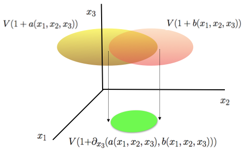
Following the above proof, $a=1$ and $b=x_{q}+x_{q}x_{r}$ (note that $\frac{\partial}{\partial x_{p}}(\pi(F))=x_{q}+x_{q}x_{r}$ ). Therefore $\Theta(a)=\top$ and $\Theta(b)=q\land\lnot r$ , so

F\equiv\lnot(\top\leftrightarrow p\land(q\land\lnot r))

The forgetting operator that we are going to define next, called independence rule, aims to represent the models of the conservative retraction as those that can be extended to models of $F\land G$ (that is, the idea behind Lifting Lemma). Geometrically, if $a$ and $b$ are the polynomials $\pi(F)$ and $\pi(G)$ respectively, then the vanishing set $V(1+a,1+b)$ (which could correspond to the set of models both of $F$ and $G$ ) is projected by $\partial_{p}$ (see Fig. 4). The algebraic expression of the projection is described as a rule.

Definition 4.4.

The independence rule (or $\partial$ -rule) on polynomial formulas is defined as follows: given $a_{1},a_{2}\in{\mathbb{F}}_{2}[{\bf x}]$ and $x$ an indeterminate

\displaystyle\hskip 14.22636pt\quad\frac{a_{1},\ a_{2}}{\partial_{x}(a_{1},a_{2})}

where $\partial_{x}(a_{1},a_{2})={1+\Phi\left[(1+a_{1}\cdot a_{2})(1+a_{1}\cdot\frac{\partial}{\partial x}a_{2}+a_{2}\cdot\frac{\partial}{\partial x}a_{1}+\frac{\partial}{\partial x}a_{1}\cdot\frac{\partial}{\partial x}a_{2})\right]}$

If $a_{i}=b_{i}+x_{p}\cdot c_{i},\ \mbox{with }\mbox{deg}_{x_{p}}(b_{i})=\mbox{deg}_{x_{p}}(c_{i})=0\ (i=1,2)$ , the rule we can rewritten as:

\partial_{x_{p}}(a_{1},a_{2})={\Phi\left[1+(1+b_{1}\cdot b_{2})[1+(b_{1}+c_{1})(b_{2}+c_{2})]\right]}

For example, to compute

a=\partial_{x_{2}}(1+x_{2}x_{3}x_{5}+x_{3}x_{5},1+x_{1}x_{2}x_{3}x_{4}x_{5}+x_{1}x_{2}x_{3}x_{5})

we take

b_{1}=1+x_{3}x_{5},\ c_{1}=x_{3}x_{5}\qquad\mbox{and }\qquad b_{2}=1,\ c_{2}=(1+x_{4})x_{1}x_{3}x_{5}

so the result is $a=1+x_{1}x_{3}x_{4}x_{5}+x_{1}x_{3}x_{5}.$

Note that independence rule is symmetric.

5 Independence rule and non-clausal theorem proving

The independence rule for formulas is defined as

$\partial_{p}(F,G):=\Theta(\partial_{x_{p}}(\pi(F),\pi(G)))$

Following with above example,

\partial_{p_{2}}(p_{3}\land p_{5}\to p_{2},p_{1}\land p_{2}\land p_{3}\land p_{5}\to p_{4})=

=\Theta(\partial_{x_{2}}(1+x_{2}x_{3}x_{5}+x_{3}x_{5},1+x_{1}x_{2}x_{3}x_{4}x_{5}+x_{1}x_{2}x_{3}x_{5}))=

=\Theta(1+x_{1}x_{3}x_{4}x_{5}+x_{1}x_{3}x_{5})=\lnot(p_{1}\land p_{3}\land p_{4}\land p_{5}\leftrightarrow p_{1}\land p_{3}\land p_{5})\equiv

\equiv p_{1}\land p_{3}\land p_{5}\to p_{4}

It is worthy to point out some interesting features of the rule $\partial_{p}$ : if $\partial_{p}(F,G)$ is a tautology, then $\partial_{p}(F,G)=\top$ , and if $\partial_{p}(F,G)$ is inconsistent then $\partial_{p}(F,G)=\bot$ . Both features are consequence of the translation to polynomials: polynomial formulas corresponds of tautologies and inconsistencies are algebraically simplified to $1$ and $0$ in ${\mathbb{F}}_{2}[{\bf x}]/{\mathbb{I}}_{2}$ , respectively. In fact, we will usually work with the polynomial projections to exploit these features.

Proposition 5.1.

$\partial_{p}$ is sound

Proof.

We have to prove $F_{1}\land F_{2}\models\partial_{p}(F_{1},F_{2})$ . Suppose that

\pi(F_{1})=b_{1}+x_{p}\cdot c_{1},\quad\pi(F_{2})=b_{2}+x_{p}\cdot c_{2}

According to Thm. 2.2.(3), it is enough to prove that

V(1+\pi(F_{1})\cdot\pi(F_{2}))\subseteq V(1+\partial_{x_{p}}(\pi(F_{1}),\pi(F_{2})))

Let ${\bf u}\in V(1+\pi(F_{1})\cdot\pi(F_{2}))\subseteq{\mathbb{F}}_{2}^{n}$ , that is,

(b_{1}+x_{p}c_{1})(b_{2}+x_{p}c_{2})\large|_{\bf x=u}=1\hskip 23.49976pt\hskip 23.49976pt({\dagger})

(the notation used here is as usual: $F(x)\large|_{x=u}$ is $F(u)$ ). Let us distinguish two cases:

1.

If the $p$ -coordinate of $\bf u$ is $0$ , then by $({\dagger})$ it follows that

$b_{1}\large|_{\bf x=u}=b_{2}\large|_{\bf x=u}=1$

Therefore $(1+b_{1}b_{2})\large|_{\bf x=u}=0$ .
2.

The $p$ -coordinate of $\bf u$ is $1$ . In this case $(b_{1}+c_{1})(b_{2}+c_{2})\large|_{\bf x=u}=1$

By examining the definition of $\partial_{p}$ we conclude in both cases that

\partial_{x_{p}}(\pi(F_{1}),\pi(F_{2}))\large|_{\bf x=u}=1

so we have that ${\bf u}\in V(1+\partial_{x_{p}}(\pi(F_{1}),\pi(F_{2})))$ . ∎

Theorem 5.2.

$\partial_{p}$ is a forgetting operator

Proof.

The goal is to prove that

[\{F_{1},F_{2}\},\mathcal{L}\setminus\{p\}]\equiv\partial_{p}(F_{1},F_{2})

Let us suppose that $F_{1},F_{2}\in Form(\mathcal{L})$ such that $\pi(F_{i})=b_{i}+x_{p}c_{i}$ $i=1,2$ with $b_{i},c_{i}$ polynomial formulas without variable $x_{p}$ . Recall that in this case the expression of the rule is

\partial_{x_{p}}(\pi(F_{1}),\pi(F_{2}))=\Phi\left((1+b_{1}\cdot b_{2})\left[1+(b_{1}+c_{1})(b_{2}+c_{2})\right]\right)

Since the soundness of $\partial_{p}$ has been proved by the previous proposition, by Corollary 3.3 it is sufficient to show that any valuation $v$ on $\mathcal{L}\setminus\{p\}$ model of $\partial_{p}(F_{1},F_{2})$ can be extended to $\hat{v}\models\{F_{1},F_{2}\}$ .

Let $v\models\partial_{p}(F_{1},F_{2})$ . Let us consider the point from ${\mathbb{F}}_{2}^{n}$ asociated to $v$ , $o_{v}$ . It follows that

	$\displaystyle o_{v}\in V(\pi(\partial_{p}(F_{1},F_{2}))+1)=V(\partial_{x_{p}}(\pi(F_{1}),\pi(F_{2}))+1)=$
	$\displaystyle=V((1+b_{1}\cdot b_{2})[1+(b_{1}+c_{1})(b_{2}+c_{2})])$

\displaystyle\left((1+b_{1}\cdot b_{2})[1+(b_{1}+c_{1})(b_{2}+c_{2})]\right)\large|_{\bf x=o_{v}}=0

In order to build the required extension $\hat{v}$ , let us distinguish two cases:

1.

If $(1+b_{1}\cdot b_{2})\large|_{\bf x=o_{v}}=0$ then $\hat{v}=v\cup\{(x_{p},0)\}\models F_{1}\land F_{2}$ .
2.

If $[1+(b_{1}+c_{1})(b_{2}+c_{2})]\large|_{\bf x=o_{v}}=0$ then

$\hat{v}=v\cup\{(x_{p},1)\}\models F_{1}\land F_{2}$

∎

With some abuse of notation, we use the same symbol, $\vdash_{\partial}$ , to denote similar notions that defined in Def. 3.6 but on polynomial formulas and rules $\partial_{x_{p}}$ . In that way we can describe $\vdash_{\partial}$ -proofs on polynomials. For example, a $\partial$ -refutation for the set $\pi[\{p\to q,q\lor r\to s,\lnot(p\to s)\}]$ is

1.

$1+x_{1}+x_{1}x_{2}\hfill[\![\pi(p\to q)]\!]$
2.

$1+(x_{2}+x_{3}+x_{2}x_{3})(1+x_{4})\hfill[\![\pi(q\lor r\to s)]\!]$
3.

$x_{1}(1+x_{4})\hfill[\![\pi(\lnot(p\to s)]\!]$
4.

$1+x_{1}+x_{3}+x_{1}x_{4}+x_{3}x_{4}+x_{1}x_{3}+x_{1}x_{3}x_{4}\hfill[\![\partial_{x_{2}}\ to(1),(2)]\!]$
5.

$0\hfill[\![\partial_{x_{1}}\ to\ (3),(4)]\!]$

Corollary 5.3.

[10]

$K$ is inconsistent if and only if $K\vdash_{\partial}\bot$ .

Proof.

It is consequence of theorems 3.7 and 5.2

∎

The result, in algebraic terms, is as follows:

Corollary 5.4.

Let $F\in Form({\mathcal{L}})$ and let $K$ be a knowledge basis. The following conditions are equivalent:

1.

$K\models F$
2.

$J_{K}\vdash_{\partial}0$

Proof.

$(1)\quad\Longrightarrow\quad(2)$ : Let us suppose $K\models F$ . Then $K+\{\lnot F\}$ is inconsistent. Since $\partial_{p}$ is refutationally complete, $K+\{\lnot F\}\vdash_{\partial}\bot$ . Thus

\{1+\pi(G)\ :\ G\in K\}\cup\{\pi(F)\}\vdash_{\partial}0

$(2)\quad\Longrightarrow\quad(1)$ : If a $\partial$ -refutation is founded on polynomials, then by above theorem $K\cup\{\lnot F\}$ is inconsistent. ∎

Remark 5.5.

To compute conservative retractions we use an implementation (in Haskell language) of $\partial_{p}$ and $\partial_{x_{p}}$ . In order to simplify the presentation, we only show the computation on polynomials (that is, the application of $\partial_{x_{p}}$ ), and we use the own propositional variables as polynomial variables (that is, we identify $p$ and $x_{p}$ ) to facilitate the readibility.

The software used in the examples and experiments can be downloaded from https://github.com/DanielRodCha/SAT-Pol

Example 5.6.

Let $G=s\to r$ and $K$ be the KB

K=\left\{\begin{array}[]{l}t\land p\leftrightarrow s\\ t\land r\to s\\ t\land q\to s\\ p\land q\land s\land t\to r\\ \end{array}\right.

To decide whether $K\models G$ -by applying location lemma- we have to compute

\partial_{\mathcal{L}\setminus\{r,s\}}[K]\equiv\partial_{p}[\partial_{q}[\partial_{t}[K]]]

*

[pqrst+pqst+1,pt+s+1,qst+qt+1,rst+rt+1] (projection)
*

[pqrs+pqs+ps+s+1, ps+s+1, 1] (forgetting t)
*

[ps+s+1, 1] (forgetting q)
*

[1] (forgetting p)

Therefore:

[K,\mathcal{L}\setminus\{r,s\}]\equiv\{\top\}\not\models G

Consider now the formula $F=p\land q\land t\to s$ . In order to decide whether $K\models F$ , by location lemma we have to compute $[K,\mathcal{L}(F)]\equiv\partial_{r}[K]$

*

[pqrst+pqst+1,pt+s+1,qst+qt+1,rst+rt+1] (projection)
*

[pqst+pqt+pt+qst+qt+s+1,pt+s+1,qst+qt+1,1] (forgetting r)

To see that $\partial_{r}[K]\models F$ it is sufficient to show that $\partial_{r}[K]\cup\{\lnot F\}$ is inconsistent. The computation is made in the projection set, by saturating the polynomial set:

*

[pt+s+1,qst+qt+1, pqst+pqt] (the retraction and $\lnot$ F)
*

[0] (applying $sat_{\partial}$ )

An approach to specify contexts in AI for reasoning is to determine which set of variables $Q\subseteq K$ provides information and which variables are irrelevant for represent the specific context. In fact, in some approaches for formalizing context-based reasoning contexts are determined by this variable set. When $K$ does not provide any specific information about the context in which it is to be used, it is natural to conclude $[K,Q]$ should only contain tautologies, that is, $\partial_{\mathcal{L}\setminus Q}[K]=\{\top\}$ . In the previous example $K$ does not provide relevant information about the context determined by $\{r,s\}$ , because $[K,\mathcal{L}\setminus\{r,s\}]=\{\top\}$ .

6 Characterization sensitive implications

In addition to its use in the design and study of the independence rule, other use of Boolean derivatives is the detection of variables that are irrelevant in a formula (or, in terms of [26], to study when a formula is independent of a variable), and more generally, when a variable is irrelevant in a formula relativized to a KB (that is, in the models of the own KB).

We will say that a variable $p$ is irrelevant in a formula $F$ (or $F$ is independent of $p$ ) if $F$ is equivalent to a formula in which $p$ does not occur. This concept can be generalized to a set of variables in the natural way, and it can be proved that a $F$ formula is independent of a set of variables $X$ if and only if $F$ is independent from each variable of $X$ (see [26]). In this paper also remarks the following result:

Proposition 6.1.

The following conditions are equivalent:

1.

$F$ is independent from $x$
2.

$F\{x/\top\}\equiv F\{x/\bot\}$
3.

$F\{x/\top\}\equiv F$
4.

$F\{x/\bot\}\equiv F$

To which we could add:

5.

$\models\lnot\frac{\partial}{\partial_{p}}(F)$

In this section we are interested in studying the notion of independence relativized to a KB. Note that it may happen that a variable may be relevant in a formula but not in the KB models we are working with. To distinguish the relativized notion from the original we will use the word sensitive.

Definition 6.2.

A formula $F$ is called sensitive in $p$ with respect to a knowledge basis $K$ if $K\not\models F\{p/\lnot p\}\leftrightarrow F$ . We say that $F$ is sensitive w.r.t. $K$ (or simply sensitive, if $K$ is fixed) if $F$ is sensitive in all its variables.

The following result habilitates the use of Gröbner basis for determining sensitiveness (by means of ideal membership test in condition (4)) or that of our interest, by means of $\partial_{p}$ -rules (condition (3)).

It is straightforward to check that:

Proposition 6.3.

Let $p\in$ var $(F)$ . The following conditions are equivalent:

1.

$F$ is sensitive in $p$ with respect to a knowledge basis $K$
2.

$K\cup\{\frac{\partial}{\partial_{p}}(F)\}$ is consistent
3.

$sat_{\partial}[K\cup\{\frac{\partial}{\partial_{p}}(F)\}]=\{\top\}$
4.

$\partial_{x_{p}}\pi(F)\notin J_{K}+{\mathbb{I}}_{2}$

Proof.

$(1)\quad\Longrightarrow\quad(2)$ : Since $K\not\models F\{p/\lnot p\}\leftrightarrow F$ , there exists $v\models K$ where $v\models\lnot(F\{p/\lnot p\}\leftrightarrow F)$ , that is, $v\models K\cup\{\frac{\partial}{\partial_{p}}(F)\}$

$(2)\quad\Longrightarrow\quad(3)$ by completeness of $\vdash_{\partial}$

$(3)\quad\Longrightarrow\quad(4)$ : Let $v\models K\cup\{\frac{\partial}{\partial_{p}}(F)\}$ (it is consistent by $(3)$ . Then $\pi(\frac{\partial}{\partial_{p}}(F))(o_{v})=1$ .

Moreover $\pi(G)(o_{v})=1$ for any $G\in K$ hence $o_{v}\in J_{K}$ . Therefore the polynomial $\frac{\partial}{\partial_{p}}\pi(F)$ does not belong to $J_{K}$

$(4)\quad\Longrightarrow\quad(1)$ : Suppose $\frac{\partial}{\partial_{x_{p}}}\pi(F)\notin J_{k}+{\mathbb{I}}_{2}$ so there exists $o\in V(J_{k})$ such that $\frac{\partial}{\partial_{x_{p}}}\pi(F)(o)\neq 0$ . Then $v_{o}\models\frac{\partial}{\partial_{p}}(F)$ and $v_{o}\models K$ . Therefore $K\cup\{\frac{\partial}{\partial_{p}}(F)\}$ is consistent, so $F$ is sensitive in $p$ w.r.t. $K$ .

∎

From the definition itself it follows that Boolean derivatives can be used to tackle the problem of sensitive arguments in implications: $F$ is not sensitive in $p$ w.r.t. $K$ iff $K\models\lnot\frac{\partial}{\partial p}F$ . In this case, there exists $G$ with var $(G)=$ var $(F)\setminus\{p\}$ such that $K\models F\leftrightarrow G$ (e.g. $F\{p/\bot\}$ ).

Example 6.4.

Lets us consider the following consistent KB as a rule-based system

K=\left\{\begin{array}[]{ll}R1:p_{1}\to p_{9}\\ R2:p_{1}\to p_{10}\\ R3:\lnot p_{2}\to p_{9}\\ R4:\lnot p_{2}\to p_{10}\\ R5:(p_{1}\land p_{7})\to p_{11}\\ R6:p_{3}\to p_{7}\\ R7:p_{3}\to p_{10}\\ R8:p_{4}\to p_{11}\\ R9:p_{5}\to p_{8}\\ R10:p_{6}\to p_{9}\\ \end{array}\right.

Let us consider as a set of potential facts (potential inputs of the system)

\mathcal{F}=\{p_{1},\dots,p_{6},\lnot p_{1},\dots,\lnot p_{6}\}

We will say that a rule $R\in K$ is sensitive in $p$ w.r.t. to $K$ and a subset of potential facts $\mathcal{C}$ if $R$ is sensitive in $p$ w.r.t. $K\cup\mathcal{C}$ . Let us compute some examples:

1.
$R1$ is sensitive in $p_{1}$ w.r.t. $K$ and the potential fact set $\{\lnot p_{2}\}$ .

$\frac{\partial}{\partial_{p_{1}}}(R1)=\theta(\frac{\partial}{\partial_{x_{1}}}(1+x_{1}(1+x_{9}))=\lnot p_{9}$

and

$K\cup\{\lnot p_{2}\}\not\models\lnot p_{9}$

This condition can be checked (by using condition $(3)$ of above proposition) showing that

$[K\cup\{\lnot p_{2}\},\{p_{9}\}]\equiv\partial_{\mathcal{L}\setminus\{p_{9}\}}[K\cup\{\lnot p_{2}\}]=\{p_{9}\}\models\lnot p_{9}$

The computation is:
- *
  
  [p1p10+p1+1, p1p11p7+p1p7+1, p1p9+p1+1, p10p2+p10+p2,
  
  p10p3+p3+1, p11p4+p4+1, p2p9+p2+p9, p2+1, p3p7+p3+1,
  
  p5p8+p5+1, p6p9+p6+1] (projection of $K\cup\{\lnot p_{2}\}$ )
- *
  
  [p10p2+p10+p2,p10p3+p3+1,p11p4+p4+1,p2p9+p2+p9, p2+1,
  
  p3p7+p3+1, p5p8+p5+1,p6p9+p6+1,1] (forgetting p1)
- *
  
  [p10p3+p3+1,p10,p11p4+p4+1,p3p7+p3+1,p5p8+p5+1,
  
  p6p9+p6+1,p9,1] (forgetting p2)
- *
  
  [p10,p11p4+p4+1,p5p8+p5+1,
  
  p6p9+p6+1,p9,1] (forgetting p3)
- *
  
  [p10,p5p8+p5+1,
  
  p6p9+p6+1,p9,1] (forgetting p4)
- *
  
  [p10,p6p9+p6+1,p9,1] (forgetting p5)
- *
  
  [p10,p9,1] (forgetting p6)
- *
  
  [p10,p9,1] (forgetting p7)
- *
  
  [p10,p9,1] (forgetting p8)
- *
  
  [p9,1] (forgetting p10)
- *
  
  [p9,1] (forgetting p11)

$R5$ is not sensitive in $p_{1}$ w.r.t. the set $\{p_{4}\}$ :

\frac{\partial}{\partial_{p_{1}}}(R_{5})=\Theta(\frac{\partial}{\partial_{x_{1}}}(1+(x_{1}x_{7})(1+x_{11})))=\Theta(x_{7}(1+x_{11}))=p_{7}\land\lnot p_{11}

and $K\cup\{p_{4}\}\not\models\frac{\partial}{\partial_{p_{1}}}(R_{5})$ . In fact

[K\cup\{p_{4}\},\{p_{7},p_{11}\}]\equiv\partial_{\mathcal{L}\setminus\{p_{7},p_{11}\}}[K\cup\{p_{4}\}]=\{p_{11}\}\models\lnot\frac{\partial}{\partial_{p_{1}}}(R_{5})

7 Some applications

We will illustrate the usefulness of the tools presented to work on different types of KRR-related tasks. For reasons of paper length we will only describe two of them.

7.1 Detecting potentially dangerous states

In [6] authors show an algebraic method for detecting potentially dangerous states in a Rule Based Expert System (RBES) whose knowledge is represented by Propositional Logic. Given $K$ made up of rules, the idea is to consider the potential facts that make $K$ to infer an unwanted value (which leads a danger or undesirable state). Formally, they specify both the set $\mathcal{F}$ of potential facts (potential input literals of the RBES) and dangerous states.

Let us consider the following example, taken from the same [6], to show that it avoids dangerous situations and $K$ from example 6.4. Let

\mathcal{F}=\{p_{1},\dots,p_{6},\lnot p_{1},\dots,\lnot p_{6}\}

and let $p_{11}$ be a warning variable of a dangerous state. We know the initial state the information $\{p_{1},\lnot p_{2}\}$ , which is a secure information because $K\cup\{p_{1},\lnot p_{2}\}\not\models p_{11}$ .

In this case the question is to detect which potential facts lead us to that dangerous state, i. e. which literals $r\in\mathcal{F}$ verifying that

K\cup\{p_{1},\lnot p_{2}\}\cup\{r\}\models p_{11}

By deduction theorem it is equivalent to decide whether

K\models p_{1}\land\lnot p_{2}\land r\to p_{11}

To apply Location Lemma it is sufficient to bear in mind that this will be true if and only if

$[K,\{p_{1},\dots p_{6}\}\cup\{p_{11}\}]\models p_{1}\land\lnot p_{2}\land r\to p_{11}$ $({\dagger}{\dagger})$

In this case,

K^{\prime}=[K,\{p_{1},\dots p_{6}\}\cup\{p_{11}\}]\equiv\partial_{\mathcal{L}\setminus(\{p_{1},\dots,p_{6},p_{11}\})}[K]

In poynomial terms, this $KB$ is represented as

J=\{\tt p1p11p3+p1p3+1,p11p4+p4+1,1\}

In order to use the results of this paper it suffices to use Deduction Theorem for reducing condition $({\dagger}{\dagger})$ to

[K,\{p_{1},\dots p_{6}\}\cup\{p_{11}\}]\cup\{p_{1},\lnot p_{2}\}\models r\to p_{11}

and, by Reductio ab absurdum we have to find variables $r$ from $\mathcal{F}$ such that

[K,\{p_{1},\dots p_{6}\}\cup\{p_{11}\}]\cup\{p_{1},\lnot p_{2},\lnot p_{11}\}\models\lnot r

Obviously $p_{1},p_{2}$ do not satisfy this.

1.

For $i=3,4$ we have $[K^{\prime},\{p_{i}\}]\equiv\{\lnot p_{i}\}$ (because the polynomial projection, computed using $J$ , is $\tt 1+pi$ ), so they are dangerous variables
2.

For $i=5,6$ we have $[K^{\prime},\{p_{i}\}]\equiv\{\top\}$ , (because the polynomial projection is $\tt 1$ ), so they are not dangerous variables

7.2 Decomposing KB for context-based reasoning

This example is taken from [12]. Let us suppose we analyze the behavior of an espresso machine whose functioning aspects are captured by the axioms enumerated in Fig. 5. The first four axioms denote that if the machine pump is OK and the pump is on, then the machine has a water supply. Alternately, the machine can be filled manually, but this never happens when the pump is on. The next four axioms denote that there is some steam if and only if the boiler is OK and it is on and there is enough water supply. The last three axioms denote that there is always either coffee or tea, and that steam and coffee (or tea) result in a hot drink. Let the knowledge base for an espresso machine described in Fig. 5. Although the example is very simple, it is very useful to show the applicability of the paper tools. We have relied on the cases of [12].

Authors in [12] obtain the partition described in Fig. 6. The languages from these partitions can be used to compute conservative retractions, in order to check the completeness of the refined KB obtained in the above-mentioned paper. We compute the conservative retractions by using operators $\partial_{p}$ defined in this paper.

$\mathcal{L}(\mathcal{A}_{1})=\{on$ _ $pump,ok$ _ $pump,water,man$ _ $fill\}$ . The analogous one in our approach, $[\mathcal{A},\mathcal{L}(\mathcal{A}_{1})]$ , is equivalent to $\mathcal{A}_{1}$ ,

[\mathcal{A},\mathcal{L}(\mathcal{A}_{1})]=\left\{\begin{array}[]{l}ok$\_$pump\land on$\_$pump\to water,\ man$\_$fill\to water,\\ man$\_$fill\to\lnot on$\_$pump,\ \lnot man$\_$fill\to on$\_$pump\end{array}\right\}

$\mathcal{L}(\mathcal{A}_{2})=\{water,on$ _ $boiler,ok$ _ $boiler,steam\}$ . The analogous one in our approach, $[\mathcal{A},\mathcal{L}(\mathcal{A}_{2})]$ , is also equivalent $\mathcal{A}_{2}$ ,

[\mathcal{A},\mathcal{L}(\mathcal{A}_{2})]=\left\{\begin{array}[]{l}steam\to ok$\_$boiler,\ steam\to on$\_$boiler,\ steam\to water,\\ ok$\_$boiler\land on$\_$boiler\land water\to steam\end{array}\right\}

Finally $\mathcal{L}(\mathcal{A}_{3})=\{steam,coffee,hot$ _ $drink,teabag\}$ . The analogous one in our approach, $[\mathcal{A},\mathcal{L}(\mathcal{A}_{3})]$ , is also equivalent to $\mathcal{A}_{3}$ ,

[\mathcal{A},\mathcal{L}(\mathcal{A}_{3})]=\left\{\begin{array}[]{l}coffee\land steam\to hot$\_$drink,\ coffee\lor teabag,\\ steam\land teabag\to hot$\_$drink,\end{array}\right\}

8 Experiments

The proposal of this paper is of a general nature and is not specialized in specific fragments of propositional logic. Nevertheless, in this section we are going to experimentally compare saturation based on the independence rule with saturation based on the basic rule of forgetting variables (see [16]), which can be applied to propositional logic without syntactic restrictions, to which we add a simplification operator (we call canonical to this rule). We will formally see this idea in the next subsection. In adition, before describing the experimental results, we will show in the second subsection a refinement of the retraction to decrease the number of rule applications (for any of them).

8.1 Canonical forgetting operator

A specific syntactic feature of the forgetting operator $\partial_{p}$ is that, if $\partial_{p}(F,G)$ is a tautology, then $\partial_{p}(F,G)=\top$ , and if $\partial_{p}(F,G)$ is inconsistent then $\delta_{p}(F,G)=\bot$ . This characteristic is a consequence of the pre- and post-processing of formulas by means of polynomial translations and vice versa. Under this translation, tautologies and inconsistencies are algebraically simplified to $\top$ and $\bot$ respectively. It would not be true for any forgetting operator in general, but at least you can achieve some simplification by eliminating occurrences of $\top,\bot$ , producing thus only reduced formulas (with no occurrences of $\top$ and $\bot$ ). For this purpose we use a simplification operator:

\sigma:Form(\mathcal{L})\to Form^{r}(\mathcal{L})

(where $Form^{r}(\mathcal{L})$ is the set of reduced formulas) defined as:

1.

$\sigma(s)=s$ if $s\in\{\top,\bot\}$ , $\sigma(\lnot\top)=\bot$ and $\sigma(\lnot\bot)=\top$ ,
2.
$\sigma(F)=F$ if $\bot$ , $\top$ do not occur in $F$ , and in other case:
1. (a)
  
  $\sigma(\top\land F)=\sigma(F)$ , $\sigma(\top\lor F)=\top$
2. (b)
  
  $\sigma(\bot\land F)=\bot$ and $\sigma(\bot\lor F)=\sigma(F)$
3. (c)
  
  $\sigma(\top\to F)=\sigma(F)$ , $\sigma(F\to\top)=\top$ , $\sigma(\bot\to F)=\top$ and $\sigma(F\to\bot)=\sigma(\lnot\sigma(F))$
4. (d)
  
  If $F,G\neq\top,\bot$ , $\sigma(F*G)=\sigma(\sigma(F)*\sigma(G))$ for $*\in\{\land,\lor,\to\}$ and $\sigma(\lnot F)=\sigma(\lnot\sigma(F))$

For example,

\sigma((\bot\to p)\land(\top\land q))=\sigma(\sigma(\bot\to p)\land\sigma(\top\land q))=\sigma(\sigma(p)\land\sigma(q))=\sigma(p\land q)=p\land q

It is straight to see that $\sigma\circ\delta\equiv\delta$ for any operator $\delta$ .

Definition 8.1.

The canonical forgetting operator for a variable $p$ is defined as

\delta_{p}^{0}=\sigma\circ\delta^{*}_{p}

where

\delta_{p}^{*}(F,G):=(F\land G)\{p/\top\}\lor(F\land G)\{p/\bot\}

Proposition 8.2.

$\delta_{p}^{0}$ is a forgetting operator for $p$

Proof.

Easy by the Lifting Lemma ∎

Example 8.3.

$F=p\to q$ and $G=p\land r\to\lnot q$ :

\begin{array}[]{ll}\delta_{p}^{0}(p\to q,p\land r\to\lnot q)&=\sigma(\delta^{*}_{p}(p\to q,p\land r\to\lnot q)\\ &=\sigma\left([(p\to q)\land(p\land r\to\lnot q)]\{p/\top\}\lor\right.\\ &\left.\qquad[(p\to q)\land(p\land r\to\lnot q)]\{p/\bot\}\right)=\\ &=\sigma\left([(\top\to q)\land(\top\land r\to\lnot q)]\lor\right.\\ &\left.\qquad[(\bot\to q)\land(\bot\land r\to\lnot q)]\right)=\\ &=\sigma\left(\sigma[(\top\to q)\land(\top\land r\to\lnot q)]\lor\right.\\ &\left.\qquad\sigma[(\bot\to q)\land(\bot\land r\to\lnot q)]\right)=\\ &=\sigma\left([q\land(r\to\lnot q)]\lor\top\right)=\top\\ \end{array}

Corollary 8.4.

Let $\delta:Form(\mathcal{L})\times Form(\mathcal{L})\to Form(\mathcal{L}\setminus\{p\})$ . The following conditions are equivalent:

1.

$\delta$ is a forgetting operator for $p$ .
2.

$\delta\equiv\delta^{0}_{p}$

8.2 Refining the process

In order to make the implementation of the realistic algorithms, we will use the following result that significantly reduces the number of applications of the variable forgetting rules in practice. Besides, using the fact that it’s symmetrical, we can even further reduce the number of applications of the operators:

Proposition 8.5.

In above conditions

\delta_{p}[K]\equiv\{F\ :\ p\mbox{ does not occur in }F\}\cup\delta_{p}[\{F\in K\ :\ p\mbox{ occurs in }F\}]

Proof.

Let us denote by $A$ the first set of formulas and by $B$ the second one. We just have to prove that $A\cup B\models\delta_{p}[K]$ .

Let $\delta_{p}(F,G)$ be a formula of $\delta_{p}[K]$ . By symmetry, it is enough to consider only three cases:

1.

$p\notin var(F)\cup var(G)$ . Then $A\models F\land G\equiv\delta_{p}(F,G)$
2.

$p\in var(G)\setminus var(F)$ . Then $A\cup B\models F\land\delta_{p}(\top,G)\equiv\delta_{p}(F,G)$
3.

$p\in var(F)\cap var(G)$ . Then $\delta_{p}(F,G)\in B$

∎

8.3 Experimental results

In this section, as an illustration, we will execute variable forgetting on a set of knowledge bases to show the efficiency of the rule proposed in this paper with respect to the canonical rule in the processing of forgetting operations (fundamentally, we will focus on the cost in space, the number of symbols used in the representation). Each experiment has been performed by randomly choosing some variables present in the knowledge base and order on them (common for both operators) and we will progressively apply the corresponding operators²² 2 Although it is irrelevant to calculate the size of the knowledge bases, to estimate the time we have used a MacBook Air with a 1.6 GHz Intel Core i5 processor and 8 GB 1600 MHz DDR3 memory. The operating system is macOS High Sierra 10.13.5. Below we describe the datasets and the results obtained.

The examples are taken from the SAT Competition 2018 website³³ 3 http://sat2018.forsyte.tuwien.ac.at. In Fig. 7 their initial size (both in propositional logic and polynomial transformed) is shown. The total time used in each dataset experiment (i.e. in the application of all the corresponding operators chosen for that experiment) for both the proposed and the canonical operator is also shown. In the following tables the results of the progressive implementation of the operators are shown.

Name	Size	Size	seconds	Space (bytes)	seconds	Space (bytes)
	form.	pol.	Can. rule	Can.	Indep.	Indep.
mp1-bsat180-648	14715	18176	6.86	1,417,335,160	3.94	1,407,227,832
unsat250	24746	31800	74.60	26,453,571,424	0.92	864,549,664
mp1-squ_any_s09x07_c27_bail_UNS	36619	60318	410.87	81,535,687,624	5.24	1,706,513,448
g2-modgen-n200-m90860q08c40-13698	236112	319913	31.55	16,500,421,928	6.58	5,153,583,936
mp1-klieber2017s-1000-023-eq	351346	416531	out of time	–	518.07	426,862,970,928
mp1-tri_ali_s11_c35_bail_UNS	37606	43493	4.34	1,510,720,256	0.48	498,118,016
mp1-Nb5T06	211656	252250	75.89	38,378,129,872	1.03	1,858,302,896

Figure 7: SAT instances used in the experiments: size (both formula and polynomial representation) and total cost using both rules

mp1-bsat180-648

	Size of KB	Size of KB
Step		(Indep.
	(canonical)	rule)
1	15428	19757
2	16900	20876
3	25131	21866
4	26839	23516
5	34908	24612
6	36735	29269
7	54530	33490
8	55231	34985
9	57073	47857
10	169330	59215
11	384996	60313

unsat250

	Size of KB	Size of KB
Step		(Indep.
	(canonical)	rule)
1	26280	34091
2	28906	35443
3	34141	35891
4	68952	37731
5	191069	39242
6	193949	40393
7	200293	54677
8	214468	56846
9	231861	61119
10	407926	62330
11	939192	64986

mp1-squ_any_s09x07_c27_bail_UNS

	Size of KB	Size of KB
Step		(Indep.
	(canonical)	rule)
1	37028	62498
2	37557	64058
3	38496	63921
4	53437	66035
5	411028	65907
6	589455	67631
7	731546	67512
8	825714	68884
9	890920	68774
10	995522	69832

g2-modgen-n200-m90860q08c40-13698

	Size of KB	Size of KB
Step		(Indep.
	(canonical)	rule)
1	237141	321926
2	242392	326062
3	290876	327171
4	319155	332485
5	3339545	334528
6	3340602	341128
7	3346440	344213
8	3362678	348381
9	3367621	373298
10	3390750	537880

mp1-klieber2017s-1000-023-eq

	Size of KB	Size of KB
Step		(Indep.
	(canonical)	rule)
1	351346	1615542
2	1176815	28418531
3	2233525	28418518
4	7599271	28418513
5	74792215	28419039
6	out of time	28419304

mp1-tri_ali_s11_c35_bail_UNS

	Size of KB	Size of KB
Step		(Indep.
	(canonical)	rule)
1	37877	44127
2	38312	44943
3	38884	44771
4	50809	44634
5	54837	48200
6	213958	48072
7	237610	51134

mp1-Nb5T06

	Size of KB	Size of KB
Step		(Indep.
	(canonical)	rule)
1	212003	252400
2	213563	252570
3	222107	252724
4	222446	252862
5	224030	253000
6	232858	253482
7	233189	253620
8	234797	254102
9	243909	254240
10	294441	254378
11	3975580	254516
12	3975911	254998
13	3977425	255136
14	3985776	255278
15	4033048	255760
16	7353991	255898
17	22919499	256036

As we have observed in the experiments, despite the fact that initially the transformation to polynomials uses slightly more space, the growth in the size of the knowledge base representation when progressively applied by the operators improves considerably the resources needed with respect to the canonical operator. Note, as we have already noted, that we have compared our operator (not restricted to a sub-language of the propositional logic) with the non-specialized operator.

9 Conclusions and future work

As we have already mentioned in the introduction, the algebraic interpretation of propositional logic represents a valuable bridge for applying algebraic techniques in KRR. In this paper we have proposed a new algebraic model to solve problems on KRR whose knowledge is represented by propositional logic. We are not concerned here about the practical computational cost of the use of independence rule, the aim of a next paper. We focused on its theoretical foundations and potential applications in KRR instead.

The main technique introduced in the paper is the use of a new rule inspired in the projection of algebraic varieties and polynomial derivatives. Also, it is justified that with Boolean derivatives is possible to determine specific cases of conditional independence, the formula-variable independence relativized to a KB. The tools have been used to solve questions related with distilling KB to obtain relatively simpler KBs to solve context-based questions.

Throughout the paper we have remarked some works related to the tools used here. These works are driven to exploit the computation and use of Gröbner Basis, whilst in this paper a new method is proposed (specific for ${\mathbb{F}}_{2}$ ).

With regard to the practical complexity of the proposed method, the application of the independence rule is reduced to the the algebraic simplification of polynomials. Its calculation appears at two levels: first in the multiplication of Boolean polynomials (or in finite fields in general), since the rule of independence is reduced to products, and second in the transformation of formulas into polynomials for a complete knowledge base.

With respect to the first question, the product of Boolean polynomials is a long-studied problem, for which refined algorithms exist (see e.g. [27]). The computational complexity of the application of the rule is irrelevant (it consists mainly of four polynomial products) compared to the second issue, the translation of formulas into polynomials. Such kind of transformation has been widely used to compile and run (using Gröbner databases) rule-based programs, for example. The problems where the polynomial interpretation of the formulas (rules, for example) of a KB is used are problems where the formulas have very limited complexity. In this type of program, the number of variables that appear in a rule is very small compared to the total number (see e.g. [28, 29, 30]). Therefore the computation of conservative retraction is feasible with our approach. Moreover, in the context of algebraic interpretation of logic reasoning, the results shown in this article allow us to replace the use of "black box" implementations (those that use a computer algebra system to compile and reason) with another also algebraic but "white box" type, which can be verified/certified. The complexity of algebraic simplifications can be high when both the number of variables is large and the number of variables that occur in each knowledge base formula is relatively high (with respect to the size of the total set of variables). However it is not common (nor advisable) in programming paradigms such as logical programming (answer set or rule-based programming), DL ontologies, etc.

With respect to the use of independence rule as SAT solver, although the rule is (refutationaly) complete, its intended use in this article is to calculate conservative retractions, and we have not presented a SAT algorithm other than the intuitive one (rule application saturation). In the GitHub repository https://github.com/DanielRodCha/SAT-Pol, variants are being developed to solve more efficiently SAT problems. With regard to the complexity of the problem of the variable forgetting in the case of propositional logic, it has been studied in considerable depth due to its relationship with the SAT problem (and, in general, with problems with Boolean functions) both for the foundations on the complete logic and for various fragments of this logic (see e.g. [26, 31]). As we have shown in the section devoted to experiments, computational cost of polynomials computations are irrelevant in practice, bearing in mind that our method is nos specialized for fragments of propositional logic, since it works on the full propositional logic. That section focuses on comparing the rule with the general rule of forgetting variables, since it does not seem appropriate to compare our proposal with other approaches specialized in fragments of propositional logic.

As future work we will intend to work in two complementary research lines. On the one hand we intend to carry out the extension to many-valued logics and their applications [4, 5, 7] as well as to tackle the knowledge forgetting problem in modal logics [22]. If the underlying logic is many-valued, the algebraic varieties of the polynomial translations of the propositions do not behave intuitively (see [1]). Therefore, we need to use an appropiate version of the the Nullstellensatz Theorem. Also, for this research line, a careful generalization of the concept of Boolean derivatives, with nice logical meaning, has to be carried out [32]. On the other hand, it is possible to use our model - in a similar way to the applications presented in the paper- for implementing expert systems based on the knowledge of different experts as in [9], for diagnosis (see [33]) or -in the behalf of authors- more promising field of inconsistency management [34].

10 Acknowledgements

This work was partially supported by TIN2013-41086-P project (Spanish Ministry of Economy and Competitiveness), co-financed with FEDER funds. We also acknowledge the reviewers and editors for their valuable comments and suggestions, which have substantially improved the content of this article.

11 References

References

[1] E. Roanes-Lozano, L. M. Laita, A. Hernando, E. Roanes-Macías, An algebraic approach to rule based expert systems, Revista de la Real Academia de Ciencias Exactas, Físicas y Naturales. Serie A. Matemáticas 104 (1) (2010) 19–40.
[2] D. Kapur, P. Narendran, An equational approach to theorem proving in first-order predicate calculus, SIGSOFT Softw. Eng. Notes 10 (4) (1985) 63–66.
[3] J. Hsiang, Refutational theorem proving using term-rewriting systems, Artif. Intell. 25 (3) (1985) 255 – 300.
[4] J. Chazarain, A. Riscos, J. Alonso, E. Briales, Multi-valued logic and gröbner bases with applications to modal logic, J. Symb. Comput. 11 (3) (1991) 181 – 194.
[5] L. M. Laita, E. Roanes-Lozano, L. de Ledesma, J. A. Alonso, A computer algebra approach to verification and deduction in many-valued knowledge systems, Soft Comput. 3 (1) (1999) 7–19.
[6] E. Roanes-Lozano, A. Hernando, L. M. Laita, E. Roanes-Macías, A gröbner bases-based approach to backward reasoning in rule based expert systems, Ann Math Artif Intel 56 (3) (2009) 297–311.
[7] A. Hernando, E. Roanes-Lozano, L. M. Laita, A polynomial model for logics with a prime power number of truth values, J. Autom. Reasoning 46 (2) (2011) 205–221.
[8] J. C. Agudelo-Agudelo, C. A. Agudelo-González, O. E. García-Quintero, On polynomial semantics for propositional logics, Journal of Applied Non-Classical Logics 26 (2) (2016) 103–125.
[9] A. Hernando, E. Roanes-Lozano, An algebraic model for implementing expert systems based on the knowledge of different experts, Math. Comput. Simulat. 107 (2015) 92 – 107.
[10] G. A. Aranda-Corral, J. Borrego-Díaz, M. M. Fernández-Lebrón, Conservative retractions of propositional logic theories by means of boolean derivatives., in: Calculemus/MKM Lect. Notes Comput. Sci., Vol. 5625, Springer, 2009, pp. 45–58.
[11] P. Blair, R. V. Guha, W. Pratt, Microtheories: An ontological engineer’s guide, Tech. rep., CyC Corp. (1992).
[12] E. Amir, S. McIlraith, Partition-based logical reasoning for first-order and propositional theories, Artif. Intell. 162 (1-2) (2005) 49–88.
[13] C. Lutz, F. Wolter, Conservative extensions in the lightweight description logic EL, in: CADE-21 Lect. Notes Comput. Sci. Vol. 4603, 2007, pp. 84–99.
[14] M. J. Hidalgo-Doblado, J. A. Alonso-Jiménez, J. Borrego-Díaz, F. Martín-Mateos, J. Ruiz-Reina, Formally verified tableau-based reasoners for a description logic, J. Autom. Reasoning 52 (3) (2014) 331–360.
[15] F. Martín-Mateos, J. Alonso, M. Hidalgo, J. Ruiz-Reina, Formal verification of a generic framework to synthetize sat-provers, J. Autom. Reasoning 32 (4) (2004) 287–313.
[16] J. Lang, P. Liberatore, P. Marquis, Conditional independence in propositional logic, Artif. Intell. 141 (1) (2002) 79 – 121.
[17] F. Lin, R. Reiter, Forget it!, in: In Proceedings of the AAAI Fall Symposium on Relevance, 1994, pp. 154–159.
[18] W. W. Bledsoe, L. M. Hines, Variable elimination and chaining in a resolution-based prover for inequalities, in: CADE Lect. Notes Comp. Sci. Vol. 87, 1980, pp. 70–87.
[19] J. Larrosa, E. Morancho, D. Niso, On the practical use of variable elimination in constraint optimization problems: ’still-life’ as a case study, J. Artif. Intell. Res. 23 (2005) 421–440.
[20] Y. Moinard, Forgetting literals with varying propositional symbols, J. Log. Comput. 17 (5) (2007) 955–982.
[21] T. Eiter, K. Wang, Semantic forgetting in answer set programming, Artif. Intell. 172 (14) (2008) 1644 – 1672.
[22] Y. Zhang, Y. Zhou, Knowledge forgetting: Properties and applications, Artif. Intell. 173 (16) (2009) 1525 – 1537.
[23] K. Su, A. Sattar, G. Lv, Y. Zhang, Variable forgetting in reasoning about knowledge, J. Artif. Intell. Res. 35 (2009) 677–716.
[24] D. A. Cox, J. Little, D. O’Shea, Ideals, Varieties, and Algorithms: An Introduction to Computational Algebraic Geometry and Commutative Algebra, 3/e (Undergraduate Texts in Mathematics), Springer-Verlag, Berlin, Heidelberg, 2007.
[25] F. Winkler, Polynomial algorithms in computer algebra, Texts and monographs in symbolic computation, Springer, Wien, New York, 1996.
[26] J. Lang, P. Liberatore, P. Marquis, Propositional independence - formula-variable independence and forgetting, J. Artif. Intell. Res. 18 (2003) 391–443.
[27] R. P. Brent, P. Gaudry, E. Thomé, P. Zimmermann, Faster multiplication in gf(2)[x], in: ANTS 2008 Lect. Notes Comput. Sci. Vol. 5011, 2008, pp. 153–166.
[28] C. Rodríguez-Solano, L. M. Laita, E. Roanes-Lozano, L. López-Corral, L. Laita, A computational system for diagnosis of depressive situations, Expert Syst. Appl. 31 (1) (2006) 47–55.
[29] C. Roncero-Clemente, E. Roanes-Lozano, A multi-criteria computer package for power transformer fault detection and diagnosis, Appl. Math. Comput. 319 (2018) 153–164.
[30] E. Roanes-Lozano, J. L. G. García, G. A. Venegas, A prototype of a RBES for personalized menus generation, Applied Mathematics and Computation 315 (2017) 615–624.
[31] J. Marques-Silva, M. Janota, C. Mencía, Minimal sets on propositional formulae. problems and reductions, Artif. Intell. 252 (2017) 22 – 50.
[32] M. Fernández-Lebrón, L. Narváez-Macarro, Hasse-schmidt derivations and coefficient fields in positive characteristics, J. Algebra 265 (1) (2003) 200 – 210.
[33] J. Piury, L. M. Laita, E. Roanes-Lozano, A. Hernando, F.-J. Piury-Alonso, J. M. Gómez-Argüelles, L. Laita, A gröbner bases-based rule based expert system for fibromyalgia diagnosis, Revista de la Real Academia de Ciencias Exactas, Fisicas y Naturales. Serie A. Matematicas 106 (2) (2012) 443–456.
[34] J. Lang, P. Marquis, Reasoning under inconsistency: A forgetting-based approach, Artif. Intell. 174 (12) (2010) 799 – 823.

A logic-algebraic tool for reasoning with Knowledge-Based SystemsThis work was partially supported by TIN2013-41086-P project (Spanish Ministry of Economy and Competitiveness), co-financed with FEDER funds.

Abstract

Keywords:

1 Introduction

2 Background

2.1 Propositional logic and conservative retraction

2.2 Propositional logic and the ring 𝔽2​[𝐱]{\mathbb{F}}_{2}[{\bf x}]

2.3 Translation from formulas and vice versa

2.4 Correspondence between valuations and points in 𝔽2n{\mathbb{F}}_{2}^{n}

2.5 Polynomial projection

2.6 Propositional Logic and polynomial ideals

Theorem 2.1.

Theorem 2.2.

Remark 2.3.

3 Conservative retractions by forgetting variables

Definition 3.1.

Lemma 3.2.

Proof.

Corollary 3.3.

Proof.

Corollary 3.4.

Proof.

3.1 Conservative retractions induced by forgetting operators

Definition 3.5.

Definition 3.6.

Theorem 3.7.

Proof.

Corollary 3.8.

Proof.

Corollary 3.9.

Proof.

4 Boolean derivatives and independence rule on polynomials

Definition 4.1.

Proposition 4.2.

Proof.

Lemma 4.3.

Proof.

Definition 4.4.

5 Independence rule and non-clausal theorem proving

Proposition 5.1.

Proof.

Theorem 5.2.

Proof.

Corollary 5.3.

Proof.

Corollary 5.4.

Proof.

Remark 5.5.

Example 5.6.

6 Characterization sensitive implications

Proposition 6.1.

Definition 6.2.

Proposition 6.3.

Proof.

Example 6.4.

7 Some applications

7.1 Detecting potentially dangerous states

7.2 Decomposing KB for context-based reasoning

8 Experiments

8.1 Canonical forgetting operator

Definition 8.1.

Proposition 8.2.

Proof.

Example 8.3.

Corollary 8.4.

8.2 Refining the process

Proposition 8.5.

Proof.

8.3 Experimental results

9 Conclusions and future work

10 Acknowledgements

11 References

References

2.2 Propositional logic and the ring ${\mathbb{F}}_{2}[{\bf x}]$

2.4 Correspondence between valuations and points in ${\mathbb{F}}_{2}^{n}$