arXiv is now an independent nonprofit! Learn more
License: arXiv.org perpetual non-exclusive license
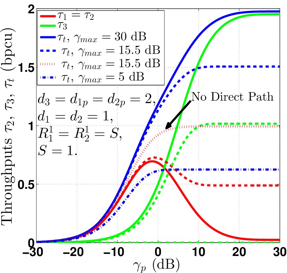
arXiv:1809.00839v1 [cs.IT] 04 Sep 2018

Framework for Discrete Rate Transmission in Buffer-Aided Underlay CRN With Direct Path

Bhupendra Kumar       Shankar Prakriya    Thanks: This work was supported by Information Technology Research Academy through sponsored project ITRA/15(63)/Mobile/MBSSCRN/01. Thanks: Bhupendra Kumar is with the Bharti School of Telecom Tech. and Management, IIT Delhi (e-mail: bkumar0810@gmail.com). S. Prakriya is with the Department of Electrical Engineering, IIT Delhi, New Delhi 110016, India (e-mail: shankar@ee.iitd.ac.in).
Abstract

In this paper, a buffered decode and forward (DF) relay based three-node underlay cooperative cognitive relay network (CRN) is considered with a direct path to the destination. The source and the relay use multiple rates, and joint rate and link selection is performed to maximize throughput. Optimum link and rate selection rules are evolved that ensure buffer stability, and expressions are derived for the throughput assuming peak power and peak interference constraints on the transmit power of the secondary nodes. The expressions are written in a manner that yields useful insights on buffer stability and role of the direct link on performance. A scheme in which the direct link signal is combined with the relayed signal is also considered, and it is demonstrated that it offers additional improvement in performance only in some scenarios. Computer simulations have been presented to verify the accuracy of derived expressions.
Keywords: Buffer-Aided Relay, Decode-and-forward, Half-Duplex, Underlay Cognitive Radio.

”This work has been submitted to an IEEE journal for possible publication. Copyright may be transferred without prior notice, after which this version may no longer be accessible”

I Introduction

Due to rapid increase in demand for data intensive applications and services, and profileration of wireless devices, the wireless industry today faces an acute spectrum shortage. Cognitive radio technologies are seen to be a solution to this shortage. Underlay type of cognitive radios, in which the transmit powers of secondary nodes is constrained to ensure that interference to the primary licensed users is below a certain interference temperature limit [1, 2], have shown great potential in increasing spectrum utilization efficiencies. Due to these constraints on the transmit powers, relays are often needed in the secondary network to increase range and reliability [3][4].

Although they incur a loss in performance as compared to full-duplex relays [5], half-duplex relays are preferred in many situations because of their simplicity. One option to overcome the loss due to half-duplex relays is to utilize rate selection, which requires channel knowledge at the transmitter[6]. In addition, when the direct link between the source and the destination is not shadowed, combining the direct and relayed signals improves performance and harnesses diversity gain in cooperative links. Yet another option to harness diversity gain is to use link selection, which requires the incorporation of a data buffer at the relay [7, 8]. Use of data buffers in relays provides some degree of freedom in scheduling links degraded by fading, and increases throughput. For this reason, buffer-aided relaying has been investigated in different scenarios extensively (relay-selection [9, 10], multi-hop [11, 12], two-way relaying [13, 14], MIMO systems[15], energy harvesting[16], physical layer security[17, 18], NOMA[19, 20], full-duplex relays [21, 22] and CRN [23, 24] etc.). Analysis of performance of buffered relays in underlay CRN has been carried out for half and full-duplex relays in [25, 26] and [27] respectively.

Motivation and Contributions

Due to the interference constraints, the link signal to noise ratios (SNRs) in underlay cognitive radio network (CRN) have large variance. For this reason, use of a buffer-aided relay with link adaptation is appealing in CRN [27][28, 29, 30]. For the same reason, use of rate selection is well motivated in CRN, and we investigate this aspect here. As noted already, due to power constraints, the nodes in underlay networks are relatively close to each other for acceptable quality of service (QoS). Taking the direct channel into consideration is therefore important in underlay CRNs. In this work, we consider the direct channel, and perform joint rate and link selection with buffered relays in a two-hop underlay cognitive network. The major contributions of our work are as follows:

  • We provide a general framework for discrete-rate transmission in underlay cognitive relay networks with a direct path. We first develop the joint rate and link-selection protocol and analyze the prerequisite for buffer stability.

  • We then rewrite the throughput in a manner that provides deep insights into performance11 1 Delay analysis is clearly of interest, but it is not included here due to paucity of space. It will be studied separately. and buffer stability.

  • We utilize the expressions to analyze throughput performance of two schemes. In the first one, joint link and rate selection is performed amongst the three links. In the second scheme, the relay and the source signal using OSTBC based on the Alamouti code whenever the R-D link is selected. To enable analysis of performance, expressions are derived for joint complementary commutative distribution function (CCDF) of instantaneous SNRs of the links for both the schemes. Note that expressions for performance of the traditional non-cognitive cooperative network follow as a special case.

II System Model

We consider a dual-hop underlay cooperative CRN as depicted in Fig.1 in which the primary network consists of a primary source (not depicted in the figure), and a primary destination (𝒫\PD). The secondary or unlicensed network consists of the secondary source (𝒮\SSS), the secondary destination (𝒟\SD), together with a half-duplex (HD) decode and forward (DF) buffer-aided secondary relay (\SR). All these nodes are assumed to possess a single antenna.

Channel Model

In this paper links 1, 2 and 3 refer to 𝒮\SSS-\SR, 𝒟\SR-\SD, and 𝒮𝒟\SSS-\SD channels respectively. The links are of fading type with coefficients hi(n)h_{i}(n), i=1,2,3i=1,2,3. The interference channels from 𝒮\SSS and \SR to 𝒫\PD are denoted by g1(n)g_{1}(n) and g2(n)g_{2}(n) respectively. We will find it convenient to define g3(n)=g1(n)g_{3}(n)=g_{1}(n). We assume Rayleigh fading channels so that hi(n)𝒞𝒩(0,Ωhi)h_{i}(n)\sim{\cal CN}\left(0,\Omega_{h_{i}}\right), and gi(n)𝒞𝒩(0,Ωgi)g_{i}(n)\sim{\cal CN}\left(0,\Omega_{g_{i}}\right), i=1,2,3i=1,2,3. Denote by 𝕀p{\mathbb{I}}_{p} the interference temperature limit (ITL) imposed by the primary network, and by max\mathbb{P}_{max} the maximum transmit power at 𝒮\SSS and \SR. We denote by γi(n)\gamma_{i}(n) the instantaneous SNR of link i,i{1,2,3}i,\,\forall i\in\{1,2,3\}. Let γmax=max/No\gamma_{max}=\mathbb{P}_{max}/N_{o}, and γp=𝕀p/No\gamma_{p}={\mathbb{I}}_{p}/N_{o}, where NoN_{o} is the power spectral density of additive white Gaussian noise samples. For underlay cognitive radio with peak transmit power (PTP) and peak interference power (PIP) constraints, γi(n)\gamma_{i}(n) is given by:

γi(n)\displaystyle\hskip-14.22636pt\gamma_{i}(n) =\displaystyle= min{γmax,γp|gi(n)|2}|hi(n)|2.\displaystyle\min\left\{\gamma_{max},\frac{\mathcal{\gamma}_{p}}{|g_{i}(n)|^{2}}\right\}|h_{i}(n)|^{2}. (1)

We assume quasi-static Rayleigh fading channels with path-loss exponent α\alpha. Hence, Ωhi=diα\Omega_{h_{i}}=d_{i}^{-\alpha} and Ωgi=dipα\Omega_{g_{i}}=d_{ip}^{-\alpha}, where did_{i} and dipd_{ip} respectively denote (for link-ii) the distances between nodes in the main and interference link . The probability pip_{i}, i{1,2}i\in\{1,2\}, that the peak interference (max|gi(n)|2\mathbb{P}_{max}|g_{i}(n)|^{2}) at 𝒫\PD is greater than 𝕀p{\mathbb{I}}_{p} when transmit power max\mathbb{P}_{max} is used, is given by [27]:

pi\displaystyle p_{i} =\displaystyle= Pr{γmax>γp|gi(n)|2}=eμi/λi,\displaystyle\Pr\left\{\gamma_{max}>\dfrac{\gamma_{p}}{|g_{i}(n)|^{2}}\right\}=e^{-{\mu_{i}}/{\lambda_{i}}}, (2)

where λi=γmaxΩhi\lambda_{i}=\gamma_{max}\,\Omega_{h_{i}} and μi=γpΩhiΩgi\mu_{i}=\frac{\gamma_{p}\Omega_{h_{i}}}{\Omega_{g_{i}}} represent the average transmit SNRs when 𝒮\SSS and \SR (respectively) transmit with powers max\mathbb{P}_{max} and 𝕀p/Ωgi\mathbb{I}_{p}/\Omega_{g_{i}}. We note once again that d3p=d1pd_{3p}=d_{1p} hence g3(n)=g1(n)g_{3}(n)=g_{1}(n) and p3=p1p_{3}=p_{1}. These notations are used for maintaining consistency in formulating the problem.

Rate Set

Joint link and rate selection is performed in this paper. We assume that 𝒮\SSS and \SR use capacity achieving codewords of single time slot and pick transmission rate RikiR_{i}^{k_{i}} when the ithi^{th} link is selected. Let Ri[0,1,,Ki]=[Ri0,Ri1,,RiKi]R_{i}^{[0,1,\ldots,K_{i}]}=[R_{i}^{0},R_{i}^{1},\ldots,R_{i}^{K_{i}}] denote the rate vector with rates arranged in increasing order so that:

Rate set{R1[0,1,k1K1]}SNR threshold set{γ1[0,1,k1K1]} for link-1 (𝒮link),Rate set{R2[0,1,k2K2]}SNR threshold set{γ2[0,1,k2K2]} for link-2 (𝒟link),Rate set{R3[0,1,k3K3]}SNR threshold set{γ3[0,1,k3K3]} for link-3 (𝒮𝒟link),\displaystyle\begin{array}[]{l}\text{Rate set}\ \{R_{1}^{[0,1,...k_{1}...K_{1}]}\}\equiv\text{SNR threshold set}\ \{\gamma_{1}^{[0,1,...k_{1}...K_{1}]}\}\text{ for link-1 }(\SSS-\SR\text{link}),\\ \text{Rate set}\ \{R_{2}^{[0,1,...k_{2}...K_{2}]}\}\equiv\text{SNR threshold set}\ \{\gamma_{2}^{[0,1,...k_{2}...K_{2}]}\}\text{ for link-2 }(\SR-\SD\text{link}),\\ \text{Rate set}\ \{R_{3}^{[0,1,...k_{3}...K_{3}]}\}\equiv\text{SNR threshold set}\ \{\gamma_{3}^{[0,1,...k_{3}...K_{3}]}\}\text{ for link-3 }(\SSS-\SD\text{link}),\end{array}

where γiki\gamma_{i}^{k_{i}} is the SNR threshold for the rate RikiR_{i}^{k_{i}}, which is defined as γiki=2Riki1\gamma_{i}^{k_{i}}=2^{R_{i}^{k_{i}}}-1. Note that the rate set for the 𝒮\SSS-\SR and 𝒮𝒟\SSS-\SD links are identical so that K1=K3K_{1}=K_{3}, and we choose a different index k3k_{3} for the third link 𝒮𝒟\SSS-\SD only for ease of exposition. Also note that initial rate is zero for every rate-set, i.e. Ri0=0R_{i}^{0}=0 hence γi0=0\gamma_{i}^{0}=0 for i{1,2,3}i\in\{1,2,3\}.

Refer to caption
Fig. 1: Three Node cognitive buffer-aided relay network.

Link Selection Variables

We will find it useful to define indicator functions that specify if a particular rate is selected for a link. Specifically, we define the 2(K1+1)+(K2+1)2(K_{1}+1)+(K_{2}+1) indicator functions uiki(n)\U_{i}^{k_{i}}(n) as follows:

uiki(n)={1Rate Riki is selected 0otherwise.i={1,2,3}\displaystyle\U_{i}^{k_{i}}(n)\hskip-2.84544pt=\hskip-2.84544pt\Bigg\{\begin{array}[]{ll}\hskip-4.26773pt1\,\,\text{Rate $R_{i}^{k_{i}}$ is selected }\\ \hskip-4.26773pt0\,\,\text{otherwise}.\end{array}i=\{1,2,3\}

Clearly, we can generate the binary link selection variables ui(n)\U_{i}(n) as follows:

ui(n)=ki=0Kiuiki(n).i{1,2,3}\displaystyle\begin{array}[]{lll}\U_{i}(n)=\sum\limits_{k_{i}=0}^{K_{i}}\U_{i}^{k_{i}}(n).\quad i\in\{1,2,3\}\end{array}

For selecting any one of the three links for transmission, we define a link selection vector as 𝐮(n)=[u1(n),u2(n),u3(n)]\mathbf{u}(n)=[\U_{1}(n),\U_{2}(n),\U_{3}(n)]. Note that i=13ui(n)=1\displaystyle\sum_{i=1}^{3}\U_{i}(n)=1 since only one rate corresponding to one link is selected.

Channel State Parameter and Set of Permissible Rates

For selection of a link, and the rate to be used on it, we clearly require information on whether the channel is in outage for that rate. These indicator variables depend on the signalling scheme. We consider two signalling schemes in this paper. For links-1 and 3, we define these indicator functions for both the signalling schemes as follows:

Iu1k1(n)={1if R1k1(n)log2(1+γ1(n))0otherwise,Iu3k3(n)={1if R3k3(n)log2(1+γ3(n))0otherwise.\displaystyle\begin{array}[]{llllll}I_{u_{1}}^{k_{1}}(n)&=&\hskip-5.69046pt\Bigg\{\begin{array}[]{ll}1\quad\text{if }R_{1}^{k_{1}}(n)\leq\,\log_{2}(1+\gamma_{1}(n))\\ 0\quad\text{otherwise,}\end{array}&\hskip-11.38092ptI_{u_{3}}^{k_{3}}(n)&=&\hskip-5.69046pt\Bigg\{\begin{array}[]{ll}1\quad\text{if }R_{3}^{k_{3}}(n)\leq\,\log_{2}(1+\gamma_{3}(n))\\ 0\quad\text{otherwise.}\end{array}\end{array}

It is apparent that Iuiki(n)Riki(n),ki=0KiI_{\U_{i}}^{k_{i}}(n)R_{i}^{k_{i}}(n),\,k_{i}=0...K_{i} can be thought of as the decodable rate set for link-ii (i=1,3i=1,3), and its maximum value Riki(n)=maxki=1,,Ki(Iuiki(n)Riki(n))R_{i}^{k_{i}^{*}}(n)=\displaystyle\max_{k_{i}=1,\ldots,K_{i}}(I_{\U_{i}}^{k_{i}}(n)R^{k_{i}}_{i}(n)) is the best feasible rate for that link. For link-2, the defintion of Iu2k2(n)I_{\U_{2}}^{k_{2}}(n) depends on the signalling scheme used. In scheme-1, when link-22 is selected (in a manner to be discussed later), the relay transmits with rate R2k2(n)=maxk2=1,,K2(Iu2k2(n)R2k2(n))R_{2}^{k_{2}^{*}}(n)=\displaystyle\max_{k_{2}=1,\ldots,K_{2}}(I_{\U_{2}}^{k_{2}}(n)R^{k_{2}}_{2}(n)). In scheme-2, both source and relay use the Alamouti orthogonal space-time block code (OSTBC) to transmit a packet to the destination when link-2 is selected, exploiting the fact that the same packets are also present at the source. Clearly, this scheme results in higher SNR at the destination.

In scheme-1, the definition follows that used for links 1 and 3 so that:

Iu2k2(n)={1if R2k2(n)log2(1+γ2(n)),0otherwise.\displaystyle I_{u_{2}}^{k_{2}}(n)=\Bigg\{\begin{array}[]{ll}1\ \ \text{if }R_{2}^{k_{2}}(n)\leq\,\log_{2}(1+\gamma_{2}(n)),\\ 0\ \ \text{otherwise.}\end{array}

In scheme-2, due to the distributed Alamouti coding, we have:

Iu2k2(n)={1if R2k2(n)log2(1+γ2(n)+γ3(n)),0otherwise.\displaystyle I_{u_{2}}^{k_{2}}(n)=\Bigg\{\begin{array}[]{ll}1\ \ \text{if }R_{2}^{k_{2}}(n)\leq\,\log_{2}(1+\gamma_{2}(n)+\gamma_{3}(n)),\\ 0\ \ \text{otherwise.}\end{array}

To facilitate scheme-2, we assume that the rate sets at the source and relay are identical, and that the source tracks the buffer-content of the relay using a feedback link. Clearly, R2k2(n)=maxk2=1,,K2(Iu2k2(n)R2k2(n))R_{2}^{k_{2}^{*}}(n)=\displaystyle\max_{k_{2}=1,\ldots,K_{2}}(I_{\U_{2}}^{k_{2}}(n)R^{k_{2}}_{2}(n)). Furthermore, since the rate sets at the source and relay are identical for scheme-2, it is clear by comparing (II) and (II) that only rates R2k2R3k3R^{k_{2}}_{2}\geq R^{k_{3}}_{3} (or equivalently index k2k3k_{2}\geq k_{3}) are permissible for scheme-2. On the contrary, scheme-1 has no such restriction due to the independence of its outage indicator functions.

Implementation of the Protocol

𝒮\SSS and \SR estimate |g1(n)|2|g_{1}(n)|^{2} and g2(n)|2g_{2}(n)|^{2} by observing reverse channel of the primary network, or using dedicated pilots transmitted by the primary receiver 𝒫{\cal P}. A pilot transmitted by 𝒟\SD enables 𝒮\SSS and \SR to estimate |h3(n)|2|h_{3}(n)|^{2} and |h2(n)|2|h_{2}(n)|^{2} respectively. Similarly, a pilot transmitted by \SR enables 𝒮\SSS to estimate |h1(n)|2|h_{1}(n)|^{2}. We therefore assume that 𝒮\SSS has knowledge of |g1(n)|2|g_{1}(n)|^{2}, |h1(n)|2|h_{1}(n)|^{2} and h3(n)|2h_{3}(n)|^{2}, and that \SR posseses knowledge |g2(n)|2|g_{2}(n)|^{2} and h2(n)|2h_{2}(n)|^{2}. Indices k1,k2k_{1}^{*},\,k_{2}^{*} and k3k_{3}^{*} of best rates of each link are selected and passed on to a control unit, which then determines the link selection that maximizes throughput.

III Implementation of Link Selection

In this section, we first formulate the throughput maximization problem and determine the optimal scheduling of reception and transmission.

Throughput Maximization

The average link-rate of link-ii over NN transmissions is given by:

τi=1Nn=1Nki=0Kiuiki(n)Iuiki(n)Riki(n).i{1,2,3}\displaystyle{}\begin{array}[]{lll}\tau_{i}&=&\dfrac{1}{N}\sum\limits_{n=1}^{N}\sum\limits_{k_{i}=0}^{K_{i}}\U_{i}^{k_{i}}(n)I_{\U_{i}}^{k_{i}}(n)R_{i}^{k_{i}}(n).\quad\forall i\in\{1,2,3\}\end{array}

The maximum feasible rate Riki(n)R_{i}^{k_{i}^{*}}(n) in link-ii is given by:

Riki(n)=maxki(Iuiki(n)Riki(n)).\displaystyle\begin{array}[]{lll}\hskip-14.22636ptR_{i}^{k_{i}^{*}}(n)=\underset{k_{i}}{\max}(I_{\U_{i}}^{k_{i}}(n)R_{i}^{k_{i}}(n)).\end{array}

We note that the system throughput τt\tau_{t} needs to be maximized (τt=τ2+τ3\tau_{t}=\tau_{2}+\tau_{3}) by suitable selection of the signalling rates and the binary link selection variables ui(n)\U_{i}(n) in an optimal fashion while ensuring buffer stability (τ1τ2\tau_{1}\leq\tau_{2}). The optimization problem can be written as22 2 We assume finite NN initially as the link and rate selection policies remain the same for both finite and infinite NN.:

maxu(n)τt=τ2+τ3 s.t. 0:τ1τ2, 1:uiki(n)(1uiki(n))=0, 2:i=13ki=0Kiuiki(n)=1.\displaystyle\begin{array}[]{lll}\hskip 144.54pt\underset{\mathbf{\mathbf{\U}}(n)}{\max}\quad{\tau}_{t}={\tau}_{2}+{\tau}_{3}\\ \text{ s.t. \hskip 28.45274pt $\C_{0}$}:\tau_{1}\leq\tau_{2},\hskip 28.45274pt\text{ $\C_{1}$}:\U_{i}^{k_{i}}(n)(1-\U_{i}^{k_{i}}(n))=0,\hskip 28.45274pt\text{ \hskip 8.5359pt$\C_{2}$}:\sum\limits_{i=1}^{3}\sum\limits_{k_{i}=0}^{K_{i}}\U_{i}^{k_{i}}(n)=1.\end{array}

Since allowing the link selection variables to take values between 00 and 11 simplifies the problem but leads to the same solution [26], we relax the binary constraint on them. We note that for infinite-size buffers, using τ1<τ2\tau_{1}<\tau_{2} for buffer stability simply leads to loss in throughput. We therefore optimize so that τ1=τ2\tau_{1}=\tau_{2}. The throughput maximization problem can then be re-written as follows:

maxu(n)τt=τ2+τ3 s.t. 0:τ1=τ2, 1a:uiki(n)0, 1b:uiki(n)1, 2a:i=13ki=0Kiuiki(n)0, 2b:i=13ki=0Kiuiki(n)1.\displaystyle\begin{array}[]{lll}\hskip 108.405pt\underset{\mathbf{\mathbf{\U}}(n)}{\max}\quad{\tau}_{t}={\tau}_{2}+{\tau}_{3}\hskip 56.9055pt\text{ s.t. \hskip 28.45274pt $\C_{0}$}:\tau_{1}=\tau_{2},\\ \text{ \hskip 0.0pt$\C_{1a}$}:\U_{i}^{k_{i}}(n)\geq 0,\text{ \hskip 8.5359pt$\C_{1b}$}:\U_{i}^{k_{i}}(n)\leq 1,\text{ \hskip 8.5359pt$\C_{2a}$}:\sum\limits_{i=1}^{3}\sum\limits_{k_{i}=0}^{K_{i}}\U_{i}^{k_{i}}(n)\geq 0,\text{ \hskip 8.5359pt$\C_{2b}$}:\sum\limits_{i=1}^{3}\sum\limits_{k_{i}=0}^{K_{i}}\U_{i}^{k_{i}}(n)\leq 1.\end{array}

where constraint 0\C_{0} is required for buffer stability, and linear constraints 1a,1b,2a\C_{1a},\,\C_{1b},\,\C_{2a} and 2b\C_{2b} arise on relaxing the binary constraint 1\C_{1} in (III).

Mode of Operation

We first note that several modes of operation arise depending on which nodes are eligible to transmit with non-zero rate. We denote by \N the mode when no link is selected to transmit (all can transmit only with rate 00), and by ~\widetilde{\N} the mode when all links can transmit at some (non-zero) rate. Similarly, mode ii arises when only link-ii can transmit at a non-zero rate, and i~\widetilde{i} implies that all links other than ii can transmit at non-zero rate. As there are a total of 33 links with 22 states (on-off) each, the number of modes is clearly 23=82^{3}=8. We represent mode by ee where e{,1,2,3,1~,2~,3~,~}{i,,i~,~}e\in\{\N,1,2,3,\widetilde{1},\widetilde{2},\widetilde{3},\widetilde{\N}\}\equiv\{i,\N,\widetilde{i},\widetilde{\N}\}. Please note that for convenience we denote the union of more than one mode, e.g. {12~3~~}\{1\cup\widetilde{2}\cup\widetilde{3}\cup\widetilde{\N}\}, which means the union of mode 11, 2~,3~,\widetilde{2},\,\widetilde{3}, and ~\widetilde{\N}, by {1,2~,3~,~}\{1,\widetilde{2},\widetilde{3},\widetilde{\N}\}.

Coin-toss Events

In situations when multiple links can transmit at a non-zero rate, the solution to the optimization problem (as discussed in what follows) invokes coin toss to select a link. In mode i~\widetilde{i}, the discrete rate Rjikj(n)R_{j\neq i}^{k_{j}}(n) for link-jj is chosen by coin toss event Cjii~(n)C_{j\neq i}^{\widetilde{i}}(n), whose probability is given as:

Pjii~=Pr{Cjii~(n)=1}.i{1,2,3}\displaystyle\begin{array}[]{lll}P_{j\neq i}^{\widetilde{i}}=\Pr\{C_{j\neq i}^{\widetilde{i}}(n)=1\}.\quad i\in\{1,2,3\}\end{array}

For example in mode 3~\widetilde{3}, where either link-11 or 22 can be selected, a choice is made between R1k1(n)R_{1}^{k_{1}^{*}}(n) and R2k2(n)R_{2}^{k_{2}^{*}}(n) by coin toss events C13~(n)C^{\widetilde{3}}_{1}(n) or C23~(n)C^{\widetilde{3}}_{2}(n), whose probabilities are P13~=Pr{C13~(n)=1}P^{\widetilde{3}}_{1}=\Pr\{C^{\widetilde{3}}_{1}(n)=1\} and P23~=Pr{C23~(n)=1}=1P13~=P¯13~P^{\widetilde{3}}_{2}=\Pr\{C^{\widetilde{3}}_{2}(n)=1\}=1-P^{\widetilde{3}}_{1}=\overline{P}^{\widetilde{3}}_{1} respectively. Similarly in mode ~\widetilde{\N}, the discrete rate Riki(n)R_{i}^{k_{i}^{*}}(n) for link-ii is chosen with the coin toss event Ci~(n)C_{i}^{\widetilde{\N}}(n), with probabilities Pi~=Pr{Ci~(n)=1}i{1,2,3}P_{i}^{\widetilde{\N}}=\Pr\{C_{i}^{\widetilde{\N}}(n)=1\}\quad i\in\{1,2,3\}.

Lagrangian dual function and variables

We now use the method of Lagrangian to perform the optimization. For convenience, we drop the time-index in uiki(n)\U_{i}^{k_{i}}(n) and Riki(n)R_{i}^{k_{i}}(n). Using Lagrange multipliers αw\alpha_{w}, βiki\beta_{i}^{k_{i}}, β~iki\tilde{\beta}^{k_{i}}_{i}, β~\tilde{\beta}_{\N} and β\beta_{\N}, we can write the Lagrangian cost function {\cal L} as:

\displaystyle\mathcal{L} =τ2τ3αw(τ1τ2)n=1N[i=13ki=0Ki[βiki{1uiki}\displaystyle=-\tau_{2}-\tau_{3}-\alpha_{w}(\tau_{1}-\tau_{2})-\sum\limits_{n=1}^{N}\Bigg[\sum\limits_{i=1}^{3}\sum\limits_{k_{i}=0}^{K_{i}}\Big[\beta_{i}^{k_{i}}\Big\{1-\U_{i}^{k_{i}}\Big\} (36a)
+β~ikiuiki]β~[1i=13ki=0Kiuiki]βi=13ki=0Kiuiki,\displaystyle\hskip 9.95863pt+\widetilde{\beta}_{i}^{k_{i}}\,\U_{i}^{k_{i}}\Big]-\widetilde{\beta}_{\N}\Big[1-\sum\limits_{i=1}^{3}\sum\limits_{k_{i}=0}^{K_{i}}\U_{i}^{k_{i}}\Big]-\beta_{\N}\sum\limits_{i=1}^{3}\sum\limits_{k_{i}=0}^{K_{i}}\U_{i}^{k_{i}},
which can also be written as follows:
\displaystyle\mathcal{L} =αwτ1(1αw)τ2τ3n=1N[i=13ki=0Kiβiki+β~]\displaystyle=-\alpha_{w}\tau_{1}-(1-\alpha_{w})\tau_{2}-\tau_{3}-\sum\limits_{n=1}^{N}\Bigg[\sum\limits_{i=1}^{3}\sum\limits_{k_{i}=0}^{K_{i}}\beta_{i}^{k_{i}}+\widetilde{\beta}_{\N}\Bigg] (36b)
+n=1Nki=0Kiuiki[i=13(βikiβ~iki)+β~β].\displaystyle\hskip 9.95863pt+\sum\limits_{n=1}^{N}\sum\limits_{k_{i}=0}^{K_{i}}\U_{i}^{k_{i}}\Bigg[\sum\limits_{i=1}^{3}(\beta_{i}^{k_{i}}-\widetilde{\beta}_{i}^{k_{i}})+\widetilde{\beta}_{\N}-\beta_{\N}\Bigg].

It is clear from the above equation that a group of Lagrangian multipliers is coupled with parameter uiki\U_{i}^{k_{i}}. Define Υiki\varUpsilon_{i}^{k_{i}} as follows:

Υiki\displaystyle{\varUpsilon_{i}^{k_{i}}} =\displaystyle= N[(βikiβ~iki)+β~β].\displaystyle N\big[(\beta_{i}^{k_{i}}-\widetilde{\beta}_{i}^{k_{i}})+\widetilde{\beta}_{\N}-\beta_{\N}\big]. (37)

Substituting the values of τ1,τ2\tau_{1},\tau_{2} and τ3\tau_{3} from (III) in the expression for \mathcal{L} in (36b), and using (37), we get:

\displaystyle\mathcal{L} =1Nn=1N[αwk1=0K1u1k1Iu1k1R1k1τ1+(1αw)k2=0K2u2k2Iu2k2R2k2τ2\displaystyle=\hskip-3.55658pt-\frac{1}{N}\sum\limits_{n=1}^{N}\Bigg[\alpha_{w}\underset{\tau_{1}}{\underbrace{\sum\limits_{k_{1}=0}^{K_{1}}\U_{1}^{k_{1}}I_{\U_{1}}^{k_{1}}R_{1}^{k_{1}}}}+(1-\alpha_{w})\underset{\tau_{2}}{\underbrace{\sum\limits_{k_{2}=0}^{K_{2}}\U_{2}^{k_{2}}I_{\U_{2}}^{k_{2}}R_{2}^{k_{2}}}} (38)
+k3=0K3u3k3Iu3k3R3k3τ3+i=13ki=0Ki(NβikiuikiΥiki)Nβ~].\displaystyle\hskip 5.69046pt+\hskip-3.55658pt\underset{\tau_{3}}{\underbrace{\sum\limits_{k_{3}=0}^{K_{3}}\U_{3}^{k_{3}}I_{\U_{3}}^{k_{3}}R_{3}^{k_{3}}}}\hskip-2.84544pt+\sum\limits_{i=1}^{3}\sum\limits_{k_{i}=0}^{K_{i}}(N\beta_{i}^{k_{i}}\hskip-3.55658pt-\U_{i}^{k_{i}}\varUpsilon_{i}^{k_{i}})\hskip-2.84544pt-N\widetilde{\beta}_{\N}\Bigg].

We note that 37 and (38) play a crucial role in the development of throughput maximization protocol.

Optimal rule for throughput maximization

Now, we next state the link selection policy.

Theorem 1: The choice of the link-ii for transmission is carried out according to (III)33 3 𝐱T{\bf x}^{T} denotes the transpose of vector 𝐱{\bf x}., which is expressed in terms of the maximality of the rate decision metrics Υiki(n)\varUpsilon_{i}^{k_{i}*}(n) given by:

Υ1k1(n)=αwR1k1(n),Υ2k2(n)=(1αw)R2k2(n),Υ3k3(n)=R3k3(n),\displaystyle\begin{array}[]{lll}\varUpsilon_{1}^{k_{1}^{*}}(n)&=&\alpha_{w^{*}}R_{1}^{k_{1}^{*}}(n),\quad\varUpsilon_{2}^{k_{2}^{*}}(n)=(1-\alpha_{w^{*}})R_{2}^{k_{2}^{*}}(n),\quad\varUpsilon_{3}^{k_{3}^{*}}(n)=R_{3}^{k_{3}^{*}}(n),\end{array}

where there exist parameter αw\alpha_{w^{*}}, and associated coin-toss probabilities44 4 We highlight the dependence of these probabilities on αw\alpha_{w}^{*} by writing these probabilities as functions of αw\alpha_{w}^{*}. Pjii~(αw)P_{j\neq i}^{\widetilde{i}}(\alpha_{w^{*}}) and Pi~(αw)P_{i}^{\widetilde{\N}}(\alpha_{w^{*}}) such that the system throughput is maximized.


u(n)[u1(n)u2(n)u3(n)]T={[000]:Υ1k1(n)=Υ2k2(n)=Υ3k3(n)=0(mode ),[100]:Υ1k1(n)>max(Υ2k2(n),Υ3k3(n))(mode 1),[010]:Υ2k2(n)>max(Υ3k3(n),Υ1k1(n))(mode 2),[001]:Υ3k3(n)>max(Υ1k1(n),Υ2k2(n))(mode 3),[0C21~(n)C31~(n)]:Υ2k2(n)=Υ3k3(n)>Υ1k1(n)(mode 1~),[C12~(n)0C32~(n)]:Υ1k1(n)=Υ3k3(n)>Υ2k2(n)(mode 2~),[C13~(n)C23~(n)0]:Υ1k1(n)=Υ2k2(n)>Υ3k3(n)(mode 3~),[C1~(n)C2~(n)C3~(n)]:Υ1k1(n)=Υ2k2(n)=Υ3k3(n)>0(mode ~).\displaystyle\begin{array}[]{lll}\hskip-9.95863pt\U(n)\hskip-2.84544pt\equiv\par\hskip-2.84544pt\left[\begin{array}[]{l l l}\hskip-5.69046ptu_{1}(n)\\ \hskip-5.69046ptu_{2}(n)\\ \hskip-5.69046ptu_{3}(n)\end{array}\hskip-2.84544pt\right]^{T}\hskip-5.69046pt=\hskip-2.84544pt\left\{\begin{array}[]{l l l}\hskip-5.69046pt[0\hskip 28.45274pt0\hskip 54.06006pt0]&:&\hskip-7.22743pt\varUpsilon_{1}^{k_{1}^{*}}(n)=\varUpsilon_{2}^{k_{2}^{*}}(n)=\varUpsilon_{3}^{k_{3}^{*}}(n)=0\ (\text{mode }\N),\\ \hskip-5.69046pt[1\hskip 28.45274pt0\hskip 54.06006pt0]&:&\hskip-7.22743pt\varUpsilon_{1}^{k_{1}^{*}}(n)>\max(\varUpsilon_{2}^{k_{2}^{*}}(n),\varUpsilon_{3}^{k_{3}^{*}}(n))\ (\text{mode }1),\\ \hskip-5.69046pt[0\hskip 28.45274pt1\hskip 54.06006pt0]&:&\hskip-7.22743pt\varUpsilon_{2}^{k_{2}^{*}}(n)>\max(\varUpsilon_{3}^{k_{3}^{*}}(n),\varUpsilon_{1}^{k_{1}^{*}}(n))\ (\text{mode }2),\\ \hskip-5.69046pt[0\hskip 28.45274pt0\hskip 54.06006pt1]&:&\hskip-7.22743pt\varUpsilon_{3}^{k_{3}^{*}}(n)>\max(\varUpsilon_{1}^{k_{1}^{*}}(n),\varUpsilon_{2}^{k_{2}^{*}}(n))\ (\text{mode }3),\\ \hskip-5.69046pt[0\hskip 28.45274ptC^{\widetilde{1}}_{2}(n)\hskip 16.50264pt{C^{\widetilde{1}}_{3}}(n)]&:&\hskip-7.22743pt\varUpsilon_{2}^{k_{2}^{*}}(n)=\varUpsilon_{3}^{k_{3}^{*}}(n)>\varUpsilon_{1}^{k_{1}^{*}}(n)\hskip 28.45274pt(\text{mode }\widetilde{1}),\\ \hskip-5.69046pt[C^{\widetilde{2}}_{1}(n)\hskip 14.22636pt0\hskip 35.56593ptC^{\widetilde{2}}_{3}(n)]&:&\hskip-7.22743pt\varUpsilon_{1}^{k_{1}^{*}}(n)=\varUpsilon_{3}^{k_{3}^{*}}(n)>\varUpsilon_{2}^{k_{2}^{*}}(n)\hskip 28.45274pt(\text{mode }\widetilde{2}),\\ \hskip-5.69046pt[C_{1}^{\widetilde{3}}(n)\hskip 13.6572ptC_{2}^{\widetilde{3}}(n)\hskip 36.41948pt0]&:&\hskip-7.22743pt\varUpsilon_{1}^{k_{1}^{*}}(n)=\varUpsilon_{2}^{k_{2}^{*}}(n)>\varUpsilon_{3}^{k_{3}^{*}}(n)\hskip 28.45274pt(\text{mode }\widetilde{3}),\\ \hskip-5.69046pt[C_{1}^{\widetilde{\N}}(n)\hskip 9.24706ptC_{2}^{\widetilde{\N}}(n)\hskip 12.80365ptC_{3}^{\widetilde{\N}}(n)]&:&\hskip-7.22743pt\varUpsilon_{1}^{k_{1}^{*}}(n)=\varUpsilon_{2}^{k_{2}^{*}}(n)=\varUpsilon_{3}^{k_{3}^{*}}(n)>0\ (\text{mode }\widetilde{\N}).\end{array}\hskip-7.11317pt\right.\end{array}


Proof: We first make the following observations about the optimization’s conditions:

1) Dual Feasibility Condition: All the Lagrange multipliers for the inequality constraints have to be non-negative, i.e. β~,β0\widetilde{\beta}_{\N},\beta_{\N}\geq 0 and βiki,β~iki0,i={1,2,3}\beta_{i}^{k_{i}},\widetilde{\beta}_{i}^{k_{i}}\geq 0,\,\forall i=\{1,2,3\}. Further, 0αw10\leq\alpha_{w}\leq 1.

2) Complementary Slackness Condition: If an inequality is inactive, i.e. the optimal solution is in the interior of the set, the corresponding Lagrangian multiplier is zero. Therefore for i={1,2,3}i=\{1,2,3\}, we obtain:

βiki[1uiki]=0,β~ikiuiki=0,β~[1i=13ki=0Kiuiki]=0,βi=13ki=0Kiuiki=0.\displaystyle\begin{array}[]{lll}\beta_{i}^{k_{i}}\Big[1-\U_{i}^{k_{i}}\Big]=0,\quad\widetilde{\beta}_{i}^{k_{i}}\,\U_{i}^{k_{i}}=0,\quad\widetilde{\beta}_{\N}\Big[1-\sum\limits_{i=1}^{3}\sum\limits_{k_{i}=0}^{K_{i}}\U_{i}^{k_{i}}\Big]=0,\quad\beta_{\N}\sum\limits_{i=1}^{3}\sum\limits_{k_{i}=0}^{K_{i}}\U_{i}^{k_{i}}=0.\end{array}

3) Stationarity w.r.t. primal variables: According to the stationary condition, differentiation w.r.t. to sub-primal variables u1k1,u2k2\U_{1}^{k_{1}},\U_{2}^{k_{2}} and u3k3\U_{3}^{k_{3}} should be zero. Hence, we get:

u1k1=Υ1k1αwIu1k1R1k1=0,u2k2=Υ2k2(1αw)Iu2k2R2k2=0,u3k3=Υ3k3Iu3k3R3k3=0.\displaystyle\frac{\partial\mathcal{L}}{\partial\U_{1}^{k_{1}}}=\varUpsilon_{1}^{k_{1}}-\alpha_{w}I_{\U_{1}}^{k_{1}}R_{1}^{k_{1}}=0,\,\,\frac{\partial\mathcal{L}}{\partial\U_{2}^{k_{2}}}=\varUpsilon_{2}^{k_{2}}-(1-\alpha_{w})I_{\U_{2}}^{k_{2}}R_{2}^{k_{2}}=0,\,\,\frac{\partial\mathcal{L}}{\partial\U_{3}^{k_{3}}}=\varUpsilon_{3}^{k_{3}}-I_{\U_{3}}^{k_{3}}R_{3}^{k_{3}}=0.

After solving the above stationary conditions, we get:

Υ1k1=αwIu1k1R1k1,Υ2k2=(1αw)Iu2k2R2k2,Υ3k3=Iu3k3R3k3.\displaystyle\begin{array}[]{lll}\varUpsilon_{1}^{k_{1}}=\alpha_{w}I_{\U_{1}}^{k_{1}}R_{1}^{k_{1}},\hskip 56.9055pt{\varUpsilon_{2}^{k_{2}}}=(1-\alpha_{w})I_{\U_{2}}^{k_{2}}R_{2}^{k_{2}},\hskip 56.9055pt\varUpsilon_{3}^{k_{3}}=I_{\U_{3}}^{k_{3}}R_{3}^{k_{3}}.\end{array}

Table-I lists the rate decision metrics for the case when either silence occurs, or one of the links is selected for transmission. It is accomplished by finding whether the relevant multipliers are active or not (using complementary slackness condition), and then using the multipliers in the stationarity condition.

Table I: Rate selection-metrics for different link-selections
ui(n)=0,i{1,2,3}\U_{i}(n)=0,\,\forall i\in\{1,2,3\} ui(n)=1,uii(n)=0\U_{i^{*}}(n)=1,\,\U_{i\neq i^{*}}(n)=0
βiki=β~=0,i{1,2,3},\beta_{i}^{k_{i}}=\widetilde{\beta}_{\N}=0,\,\forall i\in\{1,2,3\}, β~iki=βiiki=β=0,\widetilde{\beta}_{i^{*}}^{k_{i}^{*}}=\beta_{i\neq i^{*}}^{k_{i}}=\beta_{\N}=0,    βiki,β~iiki,β~>0,\beta_{i^{*}}^{k_{i}^{*}},\hskip 7.96674pt\widetilde{\beta}_{i\neq i^{*}}^{k_{i}},\hskip 7.96674pt\widetilde{\beta}_{\N}>0,
β~iki,β>0,i{1,2,3},\widetilde{\beta}_{i}^{k_{i}},\hskip 7.96674pt\beta_{\N}>0,\,\forall i\in\{1,2,3\}, Υiki=N(+βiki+β~)>0,\varUpsilon_{i^{*}}^{k_{i}^{*}}=N(+\beta_{i^{*}}^{k_{i}^{*}}+\widetilde{\beta}_{\N})>0,
Υiki=N(β~ikiβ)<0.\varUpsilon_{i}^{k_{i}}=N(-\widetilde{\beta}_{i}^{k_{i}}-\beta_{\N})<0. Υikiki=N(β~ikiki+β~)<Υiki,\varUpsilon_{i^{*}}^{k_{i}\neq k_{i}^{*}}=N(-\widetilde{\beta}_{i^{*}}^{k_{i}\neq k_{i}^{*}}+\widetilde{\beta}_{\N})<\varUpsilon_{i^{*}}^{k_{i}^{*}},\,\,\, Υiiki=N(β~iiki+β~)<Υiki.\varUpsilon_{i\neq i^{*}}^{k_{i}}=N(-\widetilde{\beta}_{i\neq i^{*}}^{k_{i}}+\widetilde{\beta}_{\N})<\varUpsilon_{i^{*}}^{k_{i}^{*}}.

Whenever silence occurs, uiki=0u_{i}^{k_{i}}=0, therefore it is clear from the Table-I that Υiki<0\varUpsilon_{i}^{k_{i}}<0, ki0k_{i}\neq 0. Since 0αw10\leq\alpha_{w}\leq 1, it is clear from (III) that silence occurs when Υi0=maxki(Υiki)=0Riki=0,i.\varUpsilon_{i}^{0}=\max_{k_{i}}(\varUpsilon_{i}^{k_{i}})=0\Rightarrow R_{i}^{k_{i}^{*}}=0,\,\forall i. Whenever one of the link i=ii=i^{*} transmits, uiki=1u_{i^{*}}^{k_{i}^{*}}=1, it is again clear from the Table-I that Υiki>0\varUpsilon_{i^{*}}^{k_{i}^{*}}>0 and Υiki>Υikiki\varUpsilon_{i^{*}}^{k_{i}^{*}}>\varUpsilon_{i^{*}}^{k_{i}\neq k_{i}^{*}} and Υiki>Υiiki\varUpsilon_{i^{*}}^{k_{i}^{*}}>\varUpsilon_{i\neq i^{*}}^{k_{i}}. Hence in order to get optimum system throughput, we take the maximum of Υiki\varUpsilon_{i}^{k_{i}} per time slot, which is expressed in terms of RikiR_{i}^{k_{i}^{*}} in (III). Now, variable αw\alpha_{w} adjusts the selection of links and rates. If for some αw\alpha_{w}, the value of two or more decision metrics are the same, the link ii^{*} among these is chosen for transmission, i.e. ui(n)=1u_{i*}(n)=1, based on the relevant coin-toss probabilities. \blacksquare

It is clear that given αw\alpha_{w}, the maximal feasible rate of either link 1, 21,\,2 or 33 is chosen if the corresponding decision-metric is greater than the decision-metric of the maximal feasible rate of other links (when there is equality, a coin toss is used to select a link). When Υiki\varUpsilon_{i}^{k_{i}*} is maximum, then its corresponding uikiu_{i}^{k_{i}^{*}} is set to unity (which also sets βiki,β~\beta_{i^{*}}^{k_{i}^{*}},\,\widetilde{\beta}_{\N} and resets β,β~iki\beta_{\N},\,\widetilde{\beta}_{i^{*}}^{k_{i}^{*}}). The choice of αw\alpha_{w^{*}} and the coin toss probabilities depend on the channel statistics and is discussed in the following sections.

IV Performance Evaluation

In this section, we express the throughput in terms of the rates obtained in various operating modes listed in (III). This will yield insights on choice of αw\alpha_{w} for buffer stability. We also describe the coin-toss probabilities and associated link-rates (buffered, direct and total) for various cases. In the second part of this section, we discuss performance with the two signalling schemes.

Average link-rate for a mode of operation

Now, in order to obtain an expression for average throughput, we need to represent the link rate of (III) in a different form. To this end, we first derive an expression for the joint probability PR1k1R2k2R3k3P_{R_{1}^{k_{1}}R_{2}^{k_{2}}R_{3}^{k_{3}}} of {R1k1,R2k2,R3k3}((k1,k2,k3))\{R_{1}^{k_{1}},R_{2}^{k_{2}},R_{3}^{k_{3}}\}\,(\equiv(k_{1},k_{2},k_{3})) being selected as the maximum permissible rates by links 11, 22 and 33 respectively in any signalling interval. It is defined as:

PR1k1R2k2R3k3\displaystyle\hskip-14.22636ptP_{R_{1}^{k_{1}}R_{2}^{k_{2}}R_{3}^{k_{3}}} =\displaystyle= Pr{maxk(Iu1kR1k)=R1k1,maxk(Iu2kR2k)=R2k2,maxk(Iu3kR3k)=R3k3}.\displaystyle\Pr\{\underset{k_{\ell}}{\max}(I_{\U_{1}}^{k_{\ell}}R_{1}^{k_{\ell}})=R_{1}^{k_{1}},\underset{k_{\ell}}{\max}(I_{\U_{2}}^{k_{\ell}}R_{2}^{k_{\ell}})=R_{2}^{k_{2}},\underset{k_{\ell}}{\max}(I_{\U_{3}}^{k_{\ell}}R_{3}^{k_{\ell}})=R_{3}^{k_{3}}\}. (57)

It is clear from (III) that link selection is associated with modes and range of indices (k1,k2,k3)(k_{1},k_{2},k_{3}), we will find it convenient to study the link-rate of link- ii associated with the mode ee, which can be expressed as follows:

ie(αw)=𝒰e(αw)PR1k1R2k2R3k3Riki,\displaystyle\mathcal{R}_{i}^{e}(\alpha_{w})=\underset{\mathcal{U}^{e}(\alpha_{w})}{\sum}\hskip-5.69046ptP_{R_{1}^{k_{1}}R_{2}^{k_{2}}R_{3}^{k_{3}}}R_{i}^{k_{i}}, (58)

where the link-rate is averaged over the domain set for the given mode ee denoted by 𝒰e(αw)\mathcal{U}^{e}(\alpha_{w}) (note that 𝒰e(αw)\mathcal{U}^{e}(\alpha_{w}) is the collection of all the index-triplets (k1,k2,k3)(k_{1},k_{2},k_{3}) associated with that mode). Hence we express the domain-set for all the possible modes as follows:

𝒰(αw){(k1,k2,k3)|αwR1k1=(1αw)R2k2=R3k3=0},𝒰i(αw){(k1,k2,k3)|Υiki>max𝑗(Υjikj)},i{1,2,3}𝒰i~(αw){(k1,k2,k3)|Υj1ikj1=Υj2ikj2>Υiki},i{1,2,3}𝒰~(αw){(k1,k2,k3)|αwR1k1=(1αw)R2k2=R3k3>0}.\displaystyle\begin{array}[]{lll}\mathcal{U}^{\N}(\alpha_{w})\equiv\{(k_{1},k_{2},k_{3})|\,\alpha_{w}R_{1}^{k_{1}}=(1-\alpha_{w})R_{2}^{k_{2}}=R_{3}^{k_{3}}=0\},\\ \mathcal{U}^{i}(\alpha_{w})\equiv\{(k_{1},k_{2},k_{3})|\,\varUpsilon_{i}^{k_{i}*}>\underset{j}{\max}(\varUpsilon_{j\neq i}^{k_{j}*})\},\ \ i\in\{1,2,3\}\\ \mathcal{U}^{\widetilde{i}}(\alpha_{w})\equiv\{(k_{1},k_{2},k_{3})|\,\varUpsilon_{j_{1}\neq i}^{k_{j_{1}}*}=\varUpsilon_{j_{2}\neq i}^{k_{j_{2}}*}>\varUpsilon_{i}^{k_{i}*}\},i\in\{1,2,3\}\\ \mathcal{U}^{\widetilde{\N}}(\alpha_{w})\equiv\{(k_{1},k_{2},k_{3})|\,\alpha_{w}R_{1}^{k_{1}}=(1-\alpha_{w})R_{2}^{k_{2}}=R_{3}^{k_{3}}>0\}.\end{array}

We will use the above to balance the buffer and to derive an expression for the total system throughput.

Set of possible discrete αw\alpha_{w} values

Refer to caption
Fig. 2: Rate triplets represented as a cubic lattice constellation for R1k1=R2k2=R3k3={0,1,2}R_{1}^{k_{1}}=R_{2}^{k_{2}}=R_{3}^{k_{3}}=\{0,1,2\} in scheme-1.
Refer to caption
Fig. 3: Rate triplets represented as a prismatic lattice constellation for R1k1=R2k2=R3k3={0,1,2}R_{1}^{k_{1}}=R_{2}^{k_{2}}=R_{3}^{k_{3}}=\{0,1,2\} in scheme-2.

Since there are set of discrete rates available at 𝒮\SSS and \SR, it can be seen from (37) and (III) that αw\alpha_{w} takes discrete values. We first observe all possible discrete values of αw\alpha_{w} from domain set 𝒰1~(αw),𝒰3~(αw)\mathcal{U}^{\widetilde{1}}(\alpha_{w}),\,\mathcal{U}^{\widetilde{3}}(\alpha_{w}) and 𝒰2~(αw)\mathcal{U}^{\widetilde{2}}(\alpha_{w}) as follows:

R3k3=(1αw)R2k2αw=1R3k3/R2k2for 𝒰1~(αw),αwR1k1=(1αw)R2k2αw=R2k2/(R2k2+R1k1)for 𝒰3~(αw),R3k3=αwR1k1αw=R3k3/R1k1for 𝒰2~(αw).\displaystyle\begin{array}[]{lll}R_{3}^{k_{3}}=(1-\alpha_{w})R_{2}^{k_{2}}&\Rightarrow&\alpha_{w}=1-R_{3}^{k_{3}}/R_{2}^{k_{2}}\quad\text{for }\mathcal{U}^{\widetilde{1}}(\alpha_{w}),\\ \alpha_{w}R_{1}^{k_{1}}=(1-\alpha_{w})R_{2}^{k_{2}}&\Rightarrow&\alpha_{w}=R_{2}^{k_{2}}/(R_{2}^{k_{2}}+R_{1}^{k_{1}})\quad\text{for }\mathcal{U}^{\widetilde{3}}(\alpha_{w}),\\ R_{3}^{k_{3}}=\alpha_{w}R_{1}^{k_{1}}&\Rightarrow&\alpha_{w}=R_{3}^{k_{3}}/R_{1}^{k_{1}}\quad\text{for }\mathcal{U}^{\widetilde{2}}(\alpha_{w}).\par\par\end{array}

We denote by Λ\Lambda the set of all possible αw\alpha_{w} values. In order to constraint 0αw10\leq\alpha_{w}\leq 1, we always choose link-33 whenever R3k3>R1k1R_{3}^{k_{3}}>R_{1}^{k_{1}} and R3k3>R2k2R_{3}^{k_{3}}>R_{2}^{k_{2}} (R3k3>max(R1k1,R2k2)R_{3}^{k_{3}}>\max(R_{1}^{k_{1}},R_{2}^{k_{2}})). We define the set of αw\alpha_{w}, i.e., Λ\Lambda as:

αwΛ\displaystyle\alpha_{w}\in{\Lambda} \displaystyle\equiv sort{1R3k3/R2k2,R2k2/(R2k2+R1k1),R3k3/R1k1:s.t.R3k3max(R1k1,R2k2)},\displaystyle\text{sort}\{1-R_{3}^{k_{3}}/R_{2}^{k_{2}},R_{2}^{k_{2}}/(R_{2}^{k_{2}}+R_{1}^{k_{1}}),R_{3}^{k_{3}}/R_{1}^{k_{1}}\hskip 14.22636pt:s.t.\,R_{3}^{k_{3}}\leq\max(R_{1}^{k_{1}},R_{2}^{k_{2}})\}, (65)
\displaystyle\equiv {α0=0,α1,α2.αW1,αW=1}.\displaystyle\{\alpha_{0}=0,\alpha_{1},\alpha_{2}....\alpha_{W-1},\alpha_{W}=1\}.

where sort{x}\text{sort}\{x\} arranges elements of set x{x} in increasing order.

Example: Consider an example with rate set R1[0,1,2]=R2[0,1,2]={0,1,2}R_{1}^{[0,1,2]}=R_{2}^{[0,1,2]}=\{0,1,2\} (rate set R3[0,1,2]=R1[0,1,2]R_{3}^{[0,1,2]}=R_{1}^{[0,1,2]} is implied). It is clear from (65) that αwΛ{0,13,12,23,1}\alpha_{w}\in{\Lambda}\equiv\{0,\frac{1}{3},\frac{1}{2},\frac{2}{3},1\}. The rate triplets can be visualized as points on a lattice constellation. Fig. 3 and 3 depict the rate triplets in the form of the constellation diagrams for scheme-1 and 2, which are in cube and prism shapes respectively. Furthermore, the regions belonging to three different links for αw\alpha_{w} equal to 1/31/3, 1/21/2, and 2/32/3 are depicted for both the schemes. Red, green and blue constellation points correspond to indices that lead to selection of link-11, 22 and 33 respectively. It is clear from the figures that the intersecting planes for 𝒰3~\mathcal{U}^{\widetilde{3}} is always OGHO, and the point (2,2,1)(2,2,1) lies on it for αw=1/2\alpha_{w}=1/2. Again for αw=1/2\alpha_{w}=1/2, the planes OAGO and OCGO belong to 𝒰2~\mathcal{U}^{\widetilde{2}} and 𝒰1~\mathcal{U}^{\widetilde{1}} respectively. For scheme-1, the planes OGHO, OAGO and OCGO generate the two rectangular pyramids for link-1 and link-2, whose bases are AGHDA and CGHFC. Any constellation point which lies inside any of the two pyramids belongs to the respective link. When we choose αw=1/3\alpha_{w}=1/3, the region belonging to link-11 is still a rectangular pyramid with base AGHDA, whereas the region belonging to link-22 changes to a trapezoidal pyramid, whose base is BCFEB. The region belonging to link-33 is the rest of the rectangular pyramid, generated by 𝒰1~\mathcal{U}^{\widetilde{1}} and 𝒰2~\mathcal{U}^{\widetilde{2}}. Similar arguments are valid for αw=2/3\alpha_{w}=2/3. For scheme-2, everything remains the same except that the rate triplets for which k2<k3k_{2}<k_{3} are no longer relevant.

Properties of link rate over domain set, i.e. ie(αw)\mathcal{R}_{i}^{e}(\alpha_{w})

We have already defined the link rate of link ii, over the domain set 𝒰e(αw){\normalsize{\mathcal{U}^{e}(\alpha_{w})}} in (58). The next lemma addresses two properties of these rates. The first property describes relations between the rates in the events involving a coin-toss, and the second investigates how rate continuity is maintained when αw\alpha_{w} changes to αw+1\alpha_{w+1} or αw1\alpha_{w-1}. These properties will be used later to determine the αw\alpha_{w} that can stabilize the buffer, and to derive throughput expressions.

Lemma 1: The link rates over the domain set have two important properties as follows:
Property 1 (Rate-equality property): The link rates over the domain sets 𝒰1~(αw),𝒰2~(αw),𝒰3~(αw)\mathcal{U}^{\widetilde{1}}(\alpha_{w}),\,\mathcal{U}^{\widetilde{2}}(\alpha_{w}),\,\mathcal{U}^{\widetilde{3}}(\alpha_{w}) and 𝒰~(αw)\mathcal{U}^{\widetilde{\N}}(\alpha_{w}), which involve coin toss satisfy the following relations:

31~(αw)=(1αw)21~(αw),32~(αw)=αw12~(αw),αw13~(αw)=(1αw)23~(αw),3~(αw)=αw1~(αw)=(1αw)2~(αw).\displaystyle\begin{array}[]{lll}\mathcal{R}^{\widetilde{1}}_{3}(\alpha_{w})&=&(1-\alpha_{w})\mathcal{R}^{\widetilde{1}}_{2}(\alpha_{w}),\,\mathcal{R}^{\widetilde{2}}_{3}(\alpha_{w})=\alpha_{w}\mathcal{R}^{\widetilde{2}}_{1}(\alpha_{w}),\\ \alpha_{w}\mathcal{R}^{\widetilde{3}}_{1}(\alpha_{w})&=&(1-\alpha_{w})\mathcal{R}^{\widetilde{3}}_{2}(\alpha_{w}),\\ \mathcal{R}^{\widetilde{\N}}_{3}(\alpha_{w})&=&\alpha_{w}\mathcal{R}^{\widetilde{\N}}_{1}(\alpha_{w})=(1-\alpha_{w})\mathcal{R}^{\widetilde{\N}}_{2}(\alpha_{w}).\end{array}

Property 2 (Rate-continuity property): For w{1,2,,W1}w\in\{1,2,...,W-1\}, the following recursive relations hold:

{1,2~,3~,~}1(αw)=11(αw+1),{2,1~,3~,~}2(αw)=22(αw1),{3,2~}3(αw)={3,1~}3(αw1),\displaystyle\begin{array}[]{lll}\mathcal{R}^{\{1,\widetilde{2},\widetilde{3},\widetilde{\N}\}}_{1}(\alpha_{w})=\mathcal{R}_{1}^{1}(\alpha_{w+1}),\quad\mathcal{R}^{\{2,\widetilde{1},\widetilde{3},\widetilde{\N}\}}_{2}(\alpha_{w})=\mathcal{R}_{2}^{2}(\alpha_{w-1}),\quad\mathcal{R}^{\{3,\widetilde{2}\}}_{3}(\alpha_{w})=\mathcal{R}^{\{3,\widetilde{1}\}}_{3}(\alpha_{w-1}),\end{array}

and we also have 1{1,2~,3~,~}(α0=0)=2{2,1~,3~,~}(αW=1)=0.\mathcal{R}^{\{1,\widetilde{2},\widetilde{3},\widetilde{\N}\}}_{1}(\alpha_{0}=0)=\mathcal{R}^{\{2,\widetilde{1},\widetilde{3},\widetilde{\N}\}}_{2}(\alpha_{W}=1)=0.
Proof: Property 1:
We prove 32~(αw)=αw12~(αw)\mathcal{R}^{\widetilde{2}}_{3}(\alpha_{w})=\alpha_{w}\mathcal{R}^{\widetilde{2}}_{1}(\alpha_{w}) first. We write 32~(αw)\mathcal{R}^{\widetilde{2}}_{3}(\alpha_{w}) from (58) as follows:

32~(αw)\displaystyle\mathcal{R}_{3}^{\widetilde{2}}(\alpha_{w}) =\displaystyle= 𝒰2~(αw)PR1k1R2k2R3k3R3k3=𝒰2~(αw)PR1k1R2k2R3k3αwR1k1=αw𝒰2~(αw)PR1k1R2k2R3k3R1k1=αw12~(αw),\displaystyle\underset{\mathcal{U}^{\widetilde{2}}(\alpha_{w})}{\sum}\hskip-5.69046ptP_{R_{1}^{k_{1}}R_{2}^{k_{2}}R_{3}^{k_{3}}}R_{3}^{k_{3}}=\underset{\mathcal{U}^{\widetilde{2}}(\alpha_{w})}{\sum}\hskip-5.69046ptP_{R_{1}^{k_{1}}R_{2}^{k_{2}}R_{3}^{k_{3}}}\alpha_{w}R_{1}^{k_{1}}=\alpha_{w}\underset{\mathcal{U}^{\widetilde{2}}(\alpha_{w})}{\sum}\hskip-5.69046ptP_{R_{1}^{k_{1}}R_{2}^{k_{2}}R_{3}^{k_{3}}}R_{1}^{k_{1}}=\alpha_{w}\mathcal{R}^{\widetilde{2}}_{1}(\alpha_{w}),

where it is clear from (IV) that the relation R3k3=αwR1k1R_{3}^{k_{3}}=\alpha_{w}R_{1}^{k_{1}} holds true for the domain set 𝒰2~(αw)\mathcal{U}^{\widetilde{2}}(\alpha_{w}). The other relations can be proved in a similar manner.

Property 2: We prove 1{1,2~,3~,~}(αw)=11(αw+1)\mathcal{R}^{\{1,\widetilde{2},\widetilde{3},\widetilde{\N}\}}_{1}(\alpha_{w})=\mathcal{R}_{1}^{1}(\alpha_{w+1}) first. It is clear from (IV) that following relation holds true:

𝒰1(αw){(k1,k2,k3)|αwR1k1>max(R3k3,(1αw)R2k2)},𝒰2~(αw){(k1,k2,k3)|αwR1k1=R3k3>(1αw)R2k2},𝒰3~(αw){(k1,k2,k3)|αwR1k1=(1αw)R2k2>R3k3},𝒰N~(αw){(k1,k2,k3)|αwR1k1=R3k3=(1αw)R2k2}.\displaystyle\begin{array}[]{lll}\mathcal{U}^{1}(\alpha_{w})\equiv\{(k_{1},k_{2},k_{3})|\,\alpha_{w}R_{1}^{k_{1}}>\max(R_{3}^{k_{3}},(1-\alpha_{w})R_{2}^{k_{2}})\},\\ \mathcal{U}^{\widetilde{2}}(\alpha_{w})\equiv\{(k_{1},k_{2},k_{3})|\,\alpha_{w}R_{1}^{k_{1}}=R_{3}^{k_{3}}>(1-\alpha_{w})R_{2}^{k_{2}}\},\\ \mathcal{U}^{\widetilde{3}}(\alpha_{w})\equiv\{(k_{1},k_{2},k_{3})|\,\alpha_{w}R_{1}^{k_{1}}=(1-\alpha_{w})R_{2}^{k_{2}}>R_{3}^{k_{3}}\},\\ \mathcal{U}^{\widetilde{N}}(\alpha_{w})\equiv\{(k_{1},k_{2},k_{3})|\,\alpha_{w}R_{1}^{k_{1}}=R_{3}^{k_{3}}=(1-\alpha_{w})R_{2}^{k_{2}}\}.\end{array}

Since αw1<αw<αw+1\alpha_{w-1}<\alpha_{w}<\alpha_{w+1}, it is apparent from the above equation that if we increase αw\alpha_{w} to αw+1\alpha_{w+1}, all these above mentioned domain-sets transform into the following single domain-set:

𝒰1(αw+1){(k1,k2,k3)|αw+1R1k1>max(R3k3,(1αw+1)R2k2)}.\displaystyle\begin{array}[]{lll}\mathcal{U}^{1}(\alpha_{w+1})&\equiv&\{(k_{1},k_{2},k_{3})|\,\alpha_{w+1}R_{1}^{k_{1}}>\max\left(R_{3}^{k_{3}},(1-\alpha_{w+1})R_{2}^{k_{2}}\right)\}.\end{array}

Hence, it is clear that 𝒰{1,2~,3~,~}(αw)\mathcal{U}^{\{1,\widetilde{2},\widetilde{3},\widetilde{\N}\}}(\alpha_{w}) and 𝒰1(αw+1)\mathcal{U}^{1}(\alpha_{w+1}) are equal sets which we denote by 𝒰1(αw+1)𝒰{1,2~,3~,~}(αw)\mathcal{U}^{1}(\alpha_{w+1})\equiv\mathcal{U}^{\{1,\widetilde{2},\widetilde{3},\widetilde{\N}\}}(\alpha_{w}). It is also clear that if α0=0\alpha_{0}=0, then 𝒰{1,2~,3~,~}(α0=0){ϕ}\mathcal{U}^{\{1,\widetilde{2},\widetilde{3},\widetilde{\N}\}}(\alpha_{0}=0)\equiv\{\phi\} holds true, where ϕ\phi is a null set. Hence, the following outcome is obvious:

𝒰{1,2~,3~,~}(αw)𝒰1(αw+1)\displaystyle\mathcal{U}^{\{1,\widetilde{2},\widetilde{3},\widetilde{\N}\}}(\alpha_{w})\equiv\mathcal{U}^{1}(\alpha_{w+1}) \displaystyle\Rightarrow 1{1,2~,3~,~}(αw)=11(αw+1);\displaystyle\mathcal{R}^{\{1,\widetilde{2},\widetilde{3},\widetilde{\N}\}}_{1}(\alpha_{w})=\mathcal{R}_{1}^{1}(\alpha_{w+1});
𝒰{1,2~,3~,~}(α0=0){ϕ}\displaystyle\mathcal{U}^{\{1,\widetilde{2},\widetilde{3},\widetilde{\N}\}}(\alpha_{0}=0)\equiv\{\phi\} \displaystyle\Rightarrow 1{1,2~,3~,~}(α0=0)=0.\displaystyle\mathcal{R}^{\{1,\widetilde{2},\widetilde{3},\widetilde{\N}\}}_{1}(\alpha_{0}=0)=0.

Similarly, other relations can be proved by the following inferences:

𝒰{2,1~,3~,~}(αw)𝒰2(αw1)\displaystyle\mathcal{U}^{\{2,\widetilde{1},\widetilde{3},\widetilde{\N}\}}(\alpha_{w})\equiv\mathcal{U}^{2}(\alpha_{w-1}) \displaystyle\Rightarrow 2{2,1~,3~,~}(αw)=22(αw1);\displaystyle\mathcal{R}^{\{2,\widetilde{1},\widetilde{3},\widetilde{\N}\}}_{2}(\alpha_{w})=\mathcal{R}_{2}^{2}(\alpha_{w-1});
𝒰{2,1~,3~,~}(αW=1){ϕ}\displaystyle\mathcal{U}^{\{2,\widetilde{1},\widetilde{3},\widetilde{\N}\}}(\alpha_{W}=1)\equiv\{\phi\} \displaystyle\Rightarrow 2{2,1~,3~,~}(αW=1)=0;\displaystyle\mathcal{R}^{\{2,\widetilde{1},\widetilde{3},\widetilde{\N}\}}_{2}(\alpha_{W}=1)=0;
𝒰{3,2~}(αw)𝒰{3,1~}(αw1)\displaystyle\mathcal{U}^{\{3,\widetilde{2}\}}(\alpha_{w})\equiv\mathcal{U}^{\{3,\widetilde{1}\}}(\alpha_{w-1}) \displaystyle\Rightarrow 3{3,2~}(αw)=3{3,1~}(αw1).w0\displaystyle\mathcal{R}^{\{3,\widetilde{2}\}}_{3}(\alpha_{w})=\mathcal{R}^{\{3,\widetilde{1}\}}_{3}(\alpha_{w-1}).w\neq 0{\tiny\blacksquare}

Example (Contd.): Consider the previous example for αw=1/2\alpha_{w}=1/2 in scheme-1 to understand these two properties. First, the following domain-sets are also evident from Fig. 3:

𝒰1(1/2){(1,0,0),(2,0,0),(2,1,0)},𝒰2(1/2){(0,1,0),(0,2,0),(1,2,0)},𝒰1~(1/2){(0,2,1),(1,2,1)},𝒰2~(1/2){(2,0,1),(2,1,1)},𝒰3~(1/2){(1,1,0),(2,2,0)},𝒰~(1/2){(2,2,1)}.\displaystyle\begin{array}[]{lll}\mathcal{U}^{1}(1/2)\equiv\{(1,0,0),(2,0,0),\,(2,1,0)\},\ \mathcal{U}^{2}(1/2)\equiv\{(0,1,0),(0,2,0),\,(1,2,0)\},\\ \mathcal{U}^{\widetilde{1}}(1/2)\equiv\{(0,2,1),\,(1,2,1)\},\,\mathcal{U}^{\widetilde{2}}(1/2)\equiv\{(2,0,1),\,(2,1,1)\},\,\mathcal{U}^{\widetilde{3}}(1/2)\equiv\{(1,1,0),\,(2,2,0)\},\\ \mathcal{U}^{\widetilde{\N}}(1/2)\equiv\{(2,2,1)\}.\end{array}

Suppose we want to validate αw13~(αw)=(1αw)23~(αw)\alpha_{w}\mathcal{R}^{\widetilde{3}}_{1}(\alpha_{w})=(1-\alpha_{w})\mathcal{R}^{\widetilde{3}}_{2}(\alpha_{w}) for α=1/2\alpha=1/2 (13~(1/2)=23~(1/2)\mathcal{R}^{\widetilde{3}}_{1}(1/2)=\mathcal{R}^{\widetilde{3}}_{2}(1/2)), which is based on the domain set 𝒰3~(αw=1/2){(1,1,0),(2,2,0)}\mathcal{U}^{\widetilde{3}}(\alpha_{w}=1/2)\equiv\{(1,1,0),\,(2,2,0)\}, the link-rates 13~(1/2)\mathcal{R}^{\widetilde{3}}_{1}(1/2) and 23~(1/2)\mathcal{R}^{\widetilde{3}}_{2}(1/2) are written as follows, and αw13~(αw)=(1αw)23~(αw)\alpha_{w}\mathcal{R}^{\widetilde{3}}_{1}(\alpha_{w})=(1-\alpha_{w})\mathcal{R}^{\widetilde{3}}_{2}(\alpha_{w}) holds for α=1/2\alpha=1/2:

13~(1/2)=PR11R21R30R11+PR12R22R30R12=P1,1,0+2P2,2,0,23~(1/2)=PR11R21R30R21+PR12R22R30R22=P1,1,0+2P2,2,0.\displaystyle\begin{array}[]{lll}\mathcal{R}^{\widetilde{3}}_{1}(1/2)=P_{R_{1}^{1}R_{2}^{1}R_{3}^{0}}R_{1}^{1}+P_{R_{1}^{2}R_{2}^{2}R_{3}^{0}}R_{1}^{2}=P_{1,1,0}+2P_{2,2,0},\\ \mathcal{R}^{\widetilde{3}}_{2}(1/2)=P_{R_{1}^{1}R_{2}^{1}R_{3}^{0}}R_{2}^{1}+P_{R_{1}^{2}R_{2}^{2}R_{3}^{0}}R_{2}^{2}=P_{1,1,0}+2P_{2,2,0}.\end{array}

From property 2, it is inferred that 𝒰1(2/3)𝒰{1,2~,3~,~}(1/2)\mathcal{U}^{1}(2/3)\equiv\mathcal{U}^{\{1,\widetilde{2},\widetilde{3},\widetilde{\N}\}}(1/2) and 𝒰2(1/3)𝒰{2,1~,3~,~}(1/2)\mathcal{U}^{2}(1/3)\equiv\mathcal{U}^{\{2,\widetilde{1},\widetilde{3},\widetilde{\N}\}}(1/2) whereas 𝒰{1,2~,3~,~}(1/2)\mathcal{U}^{\{1,\widetilde{2},\widetilde{3},\widetilde{\N}\}}(1/2) and 𝒰{2,1~,3~,~}(1/2)\mathcal{U}^{\{2,\widetilde{1},\widetilde{3},\widetilde{\N}\}}(1/2) can be written as:

𝒰{1,2~,3~,~}(1/2){(1,0,0),(2,0,0),(2,1,0)𝒰1(1/2),(2,0,1),(2,1,1)𝒰2~(1/2),(1,1,0),(2,2,0)𝒰3~(1/2),(2,2,1)𝒰~(1/2)},𝒰{2,1~,3~,~}(1/2){(0,1,0),(0,2,0),(1,2,0)𝒰2(1/2),(0,2,1),(1,2,1)𝒰1~(1/2),(1,1,0),(2,2,0)𝒰3~(1/2),(2,2,1)𝒰~(1/2)}.\displaystyle\begin{array}[]{lll}\mathcal{U}^{\{1,\widetilde{2},\widetilde{3},\widetilde{\N}\}}(1/2)\equiv\{\overbrace{(1,0,0),(2,0,0),\,(2,1,0)}^{\mathcal{U}^{1}(1/2)},\,\overbrace{(2,0,1),\,(2,1,1)}^{\mathcal{U}^{\widetilde{2}}(1/2)},\,\overbrace{(1,1,0),\,(2,2,0)}^{\mathcal{U}^{\widetilde{3}}(1/2)},\,\overbrace{(2,2,1)}^{\mathcal{U}^{\widetilde{\N}}(1/2)}\},\\ \mathcal{U}^{\{2,\widetilde{1},\widetilde{3},\widetilde{\N}\}}(1/2)\equiv\{\underbrace{(0,1,0),(0,2,0),\,(1,2,0)}_{\mathcal{U}^{2}(1/2)},\,\underbrace{(0,2,1),\,(1,2,1)}_{\mathcal{U}^{\widetilde{1}}(1/2)},\,\underbrace{(1,1,0),\,(2,2,0)}_{\mathcal{U}^{\widetilde{3}}(1/2)},\,\underbrace{(2,2,1)}_{\mathcal{U}^{\widetilde{\N}}(1/2)}\}.\end{array}

However, (2,0,1)(2,0,1) (for which k2<k3k_{2}<k_{3}) is invalid rate triplet for scheme-2 in this example.

Average link-rate for link-i

We now express the average link-rate in terms of link-rates of possible modes for link-ii. It is evident from (III) that there are several coin toss probabilities. It will be shown later in lemma-3 of this section that the overall throughput does not depend on these coin toss probabilities. Instead, these probabilities only alter individual link rates. We can associate the coin toss probabilities of mode ~\widetilde{\N} with modes 1~\widetilde{1}, 2~\widetilde{2} or with 3~\widetilde{3}. Since associating these probabilities with mode 3~\widetilde{3} might increase the buffer-usage in some cases, we associate them with modes 1~\widetilde{1} and 2~\widetilde{2} as follows:

P1~(αw)=P12~(αw)andP2~(αw)=P21~(αw).\displaystyle\begin{array}[]{lll}P^{\widetilde{\N}}_{1}(\alpha_{w})=P^{\widetilde{2}}_{1}(\alpha_{w})\quad\text{and}\quad P^{\widetilde{\N}}_{2}(\alpha_{w})=P^{\widetilde{1}}_{2}(\alpha_{w}).\end{array}

The link rate of link-ii, i.e. τi\tau_{i} for i{1,2,3}i\in\{1,2,3\}, are now expressed as follows:

τ1(αw,P11,P12~,P13~)=P11(αw)11(αw)+P12~(αw)1{2~,~}(αw)+P13~(αw)13~(αw),\displaystyle\tau_{1}(\alpha_{w},P_{1}^{1},P^{\widetilde{2}}_{1},P^{\widetilde{3}}_{1})=P^{1}_{1}(\alpha_{w})\mathcal{R}_{1}^{1}(\alpha_{w})+P^{\widetilde{2}}_{1}(\alpha_{w})\mathcal{R}^{\{\widetilde{2},\widetilde{\N}\}}_{1}(\alpha_{w})+P^{\widetilde{3}}_{1}(\alpha_{w})\mathcal{R}^{\widetilde{3}}_{1}(\alpha_{w}),
τ2(αw,P22,P21~,P23~)=P22(αw)22(αw)+P21~(αw)2{1~,~}(αw)+P23~(αw)23~(αw),\displaystyle\tau_{2}(\alpha_{w},P_{2}^{2},P^{\widetilde{1}}_{2},P^{\widetilde{3}}_{2})=P^{2}_{2}(\alpha_{w})\mathcal{R}_{2}^{2}(\alpha_{w})+P^{\widetilde{1}}_{2}(\alpha_{w})\mathcal{R}^{\{\widetilde{1},\widetilde{\N}\}}_{2}(\alpha_{w})+P^{\widetilde{3}}_{2}(\alpha_{w})\mathcal{R}^{\widetilde{3}}_{2}(\alpha_{w}), (78)
τ3(αw,P12~,P21~)=33(αw)+P¯12~(αw)32~(αw)+P¯21~(αw)31~(αw)+(P21~(αw)+P12~(αw)¯)3~(αw),\displaystyle\tau_{3}(\alpha_{w},P^{\widetilde{2}}_{1},P^{\widetilde{1}}_{2})\hskip-2.84544pt=\hskip-2.84544pt\mathcal{R}_{3}^{3}(\alpha_{w})+\overline{P}^{\widetilde{2}}_{1}(\alpha_{w})\mathcal{R}^{\widetilde{2}}_{3}(\alpha_{w})+\overline{P}^{\widetilde{1}}_{2}(\alpha_{w})\mathcal{R}^{\widetilde{1}}_{3}(\alpha_{w})+\left(\overline{P^{\widetilde{1}}_{2}(\alpha_{w})+P^{\widetilde{2}}_{1}(\alpha_{w})}\right)\mathcal{R}^{\widetilde{\N}}_{3}(\alpha_{w}),

where probabilities P11(αw)P^{1}_{1}(\alpha_{w}) and P22(αw)P^{2}_{2}(\alpha_{w}) are useful in some special scenarios described later in the paper. The above equation will be utilized (in what follows) to find an expression for the optimum system throughput and to establish the buffer-stability conditions in various scenarios.

Use cases for buffer stability

In underlay cognitive radio networks, the average SNR of a link is dependent on the forward and the interference links to the primary receiver. For this reason, asymmetry in average SNRs of links is common in a two-hop network, even when the relay is located mid-way between the source and the destination. Three use cases are clearly of interest. In case-11, link-22 is heavily attenuated, whereas in case-22, link-11 is heavily attenuated. In case-33, neither link-11 nor link-22 is heavily attenuated. We discuss buffer-balancing conditions in these use cases.

Lemma 2: The buffer is stable for αwαw\alpha_{w}\leq\alpha_{w^{*}}, with:

w={0if22(α0)<11(α1):case1W1if11(αW)<22(αW1):case2zif22(αz1)11(αz)&11(αz+1)22(αz):case3\displaystyle\begin{array}[]{lll}{w}^{*}&=&\hskip-7.11317pt\left\{\begin{array}[]{ll}0\hskip 39.83368pt\mathrm{if}\ \mathcal{R}_{2}^{2}(\alpha_{0})<\mathcal{R}_{1}^{1}(\alpha_{1})\hskip 18.49411pt\mathrm{:case\mathchar 45\relax 1}\\ W-1\quad\mathrm{if\ }\mathcal{R}_{1}^{1}(\alpha_{W})<\mathcal{R}_{2}^{2}(\alpha_{W-1})\mathrm{:case\mathchar 45\relax 2}\\ z\hskip 39.83368pt\mathrm{if\ }\mathcal{R}_{2}^{2}(\alpha_{z-1})\geq\mathcal{R}_{1}^{1}(\alpha_{z})\hskip 4.26773pt\&\,\mathcal{R}_{1}^{1}(\alpha_{z+1})\geq\mathcal{R}_{2}^{2}(\alpha_{z})\hskip 7.11317pt\mathrm{:case\mathchar 45\relax 3}\end{array}\right.\end{array}

where zz is an integer such that z{1,2,.,W1}z\in\{1,2,....,W-1\}.
Proof:
We first consider case-11 and case-22. Using the rate continuity property 2{2,1~,3~,~}(αw)=22(αw1)\mathcal{R}^{\{2,\widetilde{1},\widetilde{3},\widetilde{\N}\}}_{2}(\alpha_{w})=\mathcal{R}_{2}^{2}(\alpha_{w-1}) of (IV) with w=1w=1, we infer the following:

2{2,1~,3~,~}(α1)=22(α0)22(α1)22(α0).\displaystyle\begin{array}[]{lll}\mathcal{R}^{\{2,\widetilde{1},\widetilde{3},\widetilde{\N}\}}_{2}(\alpha_{1})&=&\mathcal{R}_{2}^{2}(\alpha_{0})\,\,\Rightarrow\,\,\mathcal{R}^{2}_{2}(\alpha_{1})\leq\mathcal{R}_{2}^{2}(\alpha_{0}).\end{array}

If we assume that link-2 is attenuated such that 22(α1)<1{1,2~,3~,~}(α1)\mathcal{R}_{2}^{2}(\alpha_{1})<\mathcal{R}_{1}^{\{1,\widetilde{2},\widetilde{3},\widetilde{\N}\}}(\alpha_{1}), then we assign all the coin-toss events to link-2, so that τ2(α1,1,0,0)=22(α1)\tau_{2}(\alpha_{1},1,0,0)=\mathcal{R}_{2}^{2}(\alpha_{1}) increases to τ2(α1,1,1,1)=2{2,1~,3~,~}(α1)\tau_{2}(\alpha_{1},1,1,1)=\mathcal{R}_{2}^{\{2,\widetilde{1},\widetilde{3},\widetilde{\N}\}}(\alpha_{1}), which is equal to R22(α0)R_{2}^{2}(\alpha_{0}). We summarize this as follows:

P12~(α1)=P¯21~(α1)=P13~(α1)=0τ1(α1,1,0,0)=11(α1),τ2(α1,1,1,1)=2{2,1~,3~,~}(α1)=22(α0),τ3(α0,0,1)=3{3,2~}(α1).\displaystyle\begin{array}[]{lll}P^{\widetilde{2}}_{1}(\alpha_{1})=\overline{P}^{\widetilde{1}}_{2}(\alpha_{1})=P^{\widetilde{3}}_{1}(\alpha_{1})=0\Rightarrow\\ \tau_{1}(\alpha_{1},1,0,0)=\mathcal{R}_{1}^{1}(\alpha_{1}),\,\,\tau_{2}(\alpha_{1},1,1,1)=\mathcal{R}_{2}^{\{2,\widetilde{1},\widetilde{3},\widetilde{\N}\}}(\alpha_{1})={\cal R}_{2}^{2}(\alpha_{0}),\,\,\tau_{3}(\alpha_{0},0,1)=\mathcal{R}_{3}^{\{3,\widetilde{2}\}}(\alpha_{1}).\end{array}

If the link-2 is so heavily attenuated that condition 22(α0)<11(α1)\mathcal{R}_{2}^{2}(\alpha_{0})<\mathcal{R}_{1}^{1}(\alpha_{1}) still holds, lowering αw\alpha_{w} further in an attempt to stabilize the buffer is not feasible since there is no inflow rate. We summarize this state as follows:

P12~(α0)=P¯21~(α0)=P13~(α0)=1τ1(α0,1,1,1)=1{1,2~,3~,~}(α0)=0,τ2(α0,1,0,0)=22(α0),τ3(α0,1,0)=3{3,1~}(α0).\displaystyle\begin{array}[]{lll}P^{\widetilde{2}}_{1}(\alpha_{0})=\overline{P}^{\widetilde{1}}_{2}(\alpha_{0})=P^{\widetilde{3}}_{1}(\alpha_{0})=1\Rightarrow\\ \tau_{1}(\alpha_{0},1,1,1)=\mathcal{R}_{1}^{\{1,\widetilde{2},\widetilde{3},\widetilde{\N}\}}(\alpha_{0})=0,\,\,\tau_{2}(\alpha_{0},1,0,0)=\mathcal{R}_{2}^{2}(\alpha_{0}),\,\,\tau_{3}(\alpha_{0},1,0)=\mathcal{R}_{3}^{\{3,\widetilde{1}\}}(\alpha_{0}).\end{array}

However, it is evident from (IV) that we can change the link selection probability P11(α1)P_{1}^{1}(\alpha_{1}) to balance the buffer. Clearly, the buffered and direct throughput of R22(α0)R_{2}^{2}(\alpha_{0}) and 3{3,1~}(α0)\mathcal{R}_{3}^{\{3,\widetilde{1}\}}(\alpha_{0}) can maximally be achieved and buffer can be balanced with α1\alpha_{1} when P11(α1)=22(α0)/11(α1)P_{1}^{1}(\alpha_{1})=\mathcal{R}_{2}^{2}(\alpha_{0})/\mathcal{R}_{1}^{1}(\alpha_{1}). Similar arguments can be given for condition 22(αw1)<11(αw)\mathcal{R}_{2}^{2}(\alpha_{w-1})<\mathcal{R}_{1}^{1}(\alpha_{w}) in case-2, when link-1 is heavily attenuated. In this case, the buffer throughput of 11(αW)\mathcal{R}_{1}^{1}(\alpha_{W}) can maximally be achieved with direct throughput 3{3,1~}(αW1)=3{3,2~}(αW)\mathcal{R}^{\{3,\widetilde{1}\}}_{3}(\alpha_{W-1})=\mathcal{R}^{\{3,\widetilde{2}\}}_{3}(\alpha_{W}), and buffer can be balanced with αW1\alpha_{W-1} when P22(αW1)=11(αW)/22(αW1)P_{2}^{2}(\alpha_{W-1})=\mathcal{R}_{1}^{1}(\alpha_{W})/\mathcal{R}_{2}^{2}(\alpha_{W-1}).

Now consider case-3, in which neither link-1 nor link-2 is heavily attenuated. It is apparent from (IV) that for some αw=αz\alpha_{w^{*}}=\alpha_{z}, if the conditions τ1(αz,1,1,1)τ2(αz,1,0,0)\tau_{1}(\alpha_{z},1,1,1)\geq\tau_{2}(\alpha_{z},1,0,0) and τ1(αz,1,0,0)τ2(αz,1,1,1)\tau_{1}(\alpha_{z},1,0,0)\leq\tau_{2}(\alpha_{z},1,1,1) are satisfied, the inflow rate is equal to that of the outflow for some combination of these coin toss probabilities. After applying the rate-continuation property for link-1 and 2 for z{1,2,,W1}z\in\{1,2,...,W-1\}, we get the following:

τ1(αz,1,1,1)={1,2~,3~,~}1(αz)=11(αz+1),τ1(αz,1,0,0)=11(αz),τ2(αz,1,1,1)={2,1~,3~,~}2(αz)=22(αz1),τ2(αz,1,0,0)=22(αz).\displaystyle\begin{array}[]{lll}\tau_{1}(\alpha_{z},1,1,1)=\mathcal{R}^{\{1,\widetilde{2},\widetilde{3},\widetilde{\N}\}}_{1}(\alpha_{z})=\mathcal{R}_{1}^{1}(\alpha_{z+1}),\quad\tau_{1}(\alpha_{z},1,0,0)=\mathcal{R}_{1}^{1}(\alpha_{z}),\\ \tau_{2}(\alpha_{z},1,1,1)=\mathcal{R}^{\{2,\widetilde{1},\widetilde{3},\widetilde{\N}\}}_{2}(\alpha_{z})=\mathcal{R}_{2}^{2}(\alpha_{z-1}),\quad\tau_{2}(\alpha_{z},1,0,0)=\mathcal{R}_{2}^{2}(\alpha_{z}).\end{array}

The following conditions hold from the above equation and the argument stated previously:

22(αz1)11(αz)and11(αz+1)22(αz),\displaystyle\begin{array}[]{lll}\mathcal{R}_{2}^{2}(\alpha_{z-1})\geq\mathcal{R}_{1}^{1}(\alpha_{z})\quad\text{and}\quad\mathcal{R}_{1}^{1}(\alpha_{z+1})\geq\mathcal{R}_{2}^{2}(\alpha_{z}),\end{array}

which is given by (IV). Now we establish two recursions:

22(αz1)11(αz)𝑙22(αz1)1{1,2~,3~,~}(αz1)𝑚2{2,1~,3~,~}(αz1)11(αz1)𝑙22(αz2)11(αz1),\displaystyle\begin{array}[]{lll}\mathcal{R}_{2}^{2}(\alpha_{z-1})\geq\mathcal{R}_{1}^{1}(\alpha_{z})\overset{l}{\Leftrightarrow}\,\,\mathcal{R}_{2}^{2}(\alpha_{z-1})\geq\mathcal{R}_{1}^{\{1,\widetilde{2},\widetilde{3},\widetilde{\N}\}}(\alpha_{z-1})\\ \overset{m}{\Rightarrow}\,\,\mathcal{R}_{2}^{\{2,\widetilde{1},\widetilde{3},\widetilde{\N}\}}(\alpha_{z-1})\geq\mathcal{R}_{1}^{1}(\alpha_{z-1})\overset{l}{\Leftrightarrow}\,\,\mathcal{R}_{2}^{2}(\alpha_{z-2})\geq\mathcal{R}_{1}^{1}(\alpha_{z-1}),\end{array}
11(αz+1)22(αz)𝑙11(αz+1)2{2,1~,3~,}(αz+1)𝑚1{1,2~,3~,}(αz+1)22(αz+1)𝑙11(αz+2)22(αz+1),\displaystyle\begin{array}[]{lll}\mathcal{R}_{1}^{1}(\alpha_{z+1})\geq\mathcal{R}_{2}^{2}(\alpha_{z})\overset{l}{\Leftrightarrow}\,\,\mathcal{R}_{1}^{1}(\alpha_{z+1})\geq\mathcal{R}_{2}^{\{2,\widetilde{1},\widetilde{3},\N\}}(\alpha_{z+1})\\ \overset{m}{\Rightarrow}\,\,\mathcal{R}_{1}^{\{1,\widetilde{2},\widetilde{3},\N\}}(\alpha_{z+1})\geq\mathcal{R}_{2}^{2}(\alpha_{z+1})\overset{l}{\Leftrightarrow}\,\,\mathcal{R}_{1}^{1}(\alpha_{z+2})\geq\mathcal{R}_{2}^{2}(\alpha_{z+1}),\end{array}

where ll is implied by the rate-continuity property and mm due to change in coin-toss probabilities P12~(αz)P^{\widetilde{2}}_{1}(\alpha_{z}), P¯21~(αz),P13~(αz)\overline{P}^{\widetilde{1}}_{2}(\alpha_{z}),\,P^{\widetilde{3}}_{1}(\alpha_{z}) from 1 to 0 or 0 to 1. It is clear from the above recursions that 22(αz2)11(αz1)\mathcal{R}_{2}^{2}(\alpha_{z-2})\geq\mathcal{R}_{1}^{1}(\alpha_{z-1}) and 11(αz+2)22(αz+1)\mathcal{R}_{1}^{1}(\alpha_{z+2})\geq\mathcal{R}_{2}^{2}(\alpha_{z+1}). Hence, it is evident that the following will clearly hold true:

22(α0)11(α1)and11(αW)22(αW1),\displaystyle\begin{array}[]{lll}\mathcal{R}_{2}^{2}(\alpha_{0})\geq\mathcal{R}_{1}^{1}(\alpha_{1})\quad\text{and}\quad\mathcal{R}_{1}^{1}(\alpha_{W})\geq\mathcal{R}_{2}^{2}(\alpha_{W-1}),\end{array}

Note that the above contradict conditions for case-1 and case-2. This shows that when case-3 holds, case-1 and 2 can be ruled out. Now, in order to show that αz\alpha_{z} is unique, we re-write the conditions for αz1\alpha_{z-1}, αz\alpha_{z}, and αz+1\alpha_{z+1} together as follows:

22(αz2)11(αz1)and11(αz)22(αz1), for αz1,22(αz1)11(αz)and11(αz+1)22(αz), for αz,22(αz)11(αz+1)and11(αz+2)22(αz+1), for αz+1.\displaystyle\begin{array}[]{lll}\mathcal{R}_{2}^{2}(\alpha_{z-2})\geq\mathcal{R}_{1}^{1}(\alpha_{z-1})\quad\text{and}\quad\mathcal{R}_{1}^{1}(\alpha_{z})\geq\mathcal{R}_{2}^{2}(\alpha_{z-1}),\text{ for }\alpha_{z-1},\\ \mathcal{R}_{2}^{2}(\alpha_{z-1})\geq\mathcal{R}_{1}^{1}(\alpha_{z})\quad\text{and}\quad\mathcal{R}_{1}^{1}(\alpha_{z+1})\geq\mathcal{R}_{2}^{2}(\alpha_{z}),\quad\text{ for }\alpha_{z},\\ \mathcal{R}_{2}^{2}(\alpha_{z})\geq\mathcal{R}_{1}^{1}(\alpha_{z+1})\quad\text{and}\quad\mathcal{R}_{1}^{1}(\alpha_{z+2})\geq\mathcal{R}_{2}^{2}(\alpha_{z+1}),\text{ for }\alpha_{z+1}.\end{array}

It is clear from the above that when the middle equation for αz\alpha_{z} holds, the other two cannot hold simultaneously (the conditions are contradictory). Following these arguments, it can therefore be inferred that case-3 condition is indeed satisfied by a unique αz\alpha_{z} only. \blacksquare

Expression for optimum system throughput τt\tau_{t}

Now, in the next lemma we present an expression for optimum system throughput for the given system model, which is valid for both the used schemes.

Lemma 3: The average throughput of the system can be written in a simplified form as:

τt=minαwΛ(αw1{1,2~,~,3~}(αw)+(1αw)22(αw)+3{3,1~}(αw)),wW=minαwΛ(αw11(αw)+(1αw)2{2,1~,~,3~}(αw)+3{3,2~}(αw)).w0\displaystyle\begin{array}[]{lll}\hskip 0.0pt\tau_{t}&=&\underset{\alpha_{w}\in\Lambda}{\min}\Big(\alpha_{w}\mathcal{R}^{\{1,\widetilde{2},\widetilde{\N},\widetilde{3}\}}_{1}(\alpha_{w})+(1-\alpha_{w})\mathcal{R}_{2}^{2}(\alpha_{w})+\mathcal{R}^{\{3,\widetilde{1}\}}_{3}(\alpha_{w})\Big),\quad w\neq W\\ &=&\underset{\alpha_{w}\in\Lambda}{\min}\Big(\alpha_{w}\mathcal{R}_{1}^{1}(\alpha_{w})+(1-\alpha_{w})\mathcal{R}^{\{2,\widetilde{1},\widetilde{\N},\widetilde{3}\}}_{2}(\alpha_{w})+\mathcal{R}^{\{3,\widetilde{2}\}}_{3}(\alpha_{w})\Big).\quad w\neq 0\end{array}

Proof: Please see Appendix A.\blacksquare

Remark 1: It is clear from (IV) that in calculating the optimum average rate of the system, the inflow, outflow and direct link rates are weighed by αw, 1αw\alpha_{w^{*}},\,1-\alpha_{w^{*}} and 11 due to buffer balancing. The optimum value of αw\alpha_{w} was deterxmined using lemma-2. It should be noted that (IV) can also be used to determine the optimum value of αw\alpha_{w} by looking for the value of αw\alpha_{w} for which the terms in the brackets of right-hand side is minimized.

Remark 2: There are many combinations of coin-toss probabilities which leads to the same optimum solution of system throughput with a balanced buffer. The optimum throughput of the balanced buffer and the direct path might change, but optimum system throughput remains the same for these coin-toss probability combinations. It is apparent from (38) that coin-toss probabilities assist in balancing the buffer, not in maximizing throughput of the system.
we now discuss the buffered/direct throughput and coin-toss probabilities next.

Expression of coin-toss probabilities and link throughput

There exist more than one unique combination of coin-toss probabilities that yield the same optimum system throughput. For case-1 and 2, we have already discussed about the choice of P11(α1)P^{1}_{1}(\alpha_{1}) and P22(αW1)P^{2}_{2}(\alpha_{W-1}) and the relevant buffered/direct-link throughput. We now provide some analytical expressions for coin-toss probabilities in case-3. The buffer is balanced by suitable choice of P13~(αz)P^{\widetilde{3}}_{1}(\alpha_{z}) (and thereby P23~(αz)=1P13~(αz)P^{\widetilde{3}}_{2}(\alpha_{z})=1-P^{\widetilde{3}}_{1}(\alpha_{z})) when either link-1 or link-2 are relatively weak (while not being weak enough to belong to case-1 or case-2 ). Three subcases arise as listed in Table II. In case-3a, link-2 is relatively weak so that 11(αz)2{2~,3~}(αz){\cal R}_{1}^{1}(\alpha_{z})\geq{\cal R}_{2}^{\{\widetilde{2},\widetilde{3}\}}(\alpha_{z}) and 1{1,3~}(αz)22(αz){\cal R}_{1}^{\{1,\widetilde{3}\}}(\alpha_{z})\geq{\cal R}_{2}^{2}(\alpha_{z}). In this case, we set both P12~(αz)P^{\widetilde{2}}_{1}(\alpha_{z}) and P21~(αz)P^{\widetilde{1}}_{2}(\alpha_{z}) to zero and use P13~(αz)P^{\widetilde{3}}_{1}(\alpha_{z}) (and thereby P23~(αz)P^{\widetilde{3}}_{2}(\alpha_{z})) to balance the buffer (note that this might reduce throughput of the direct path). The choice of P12~(αz)P_{1}^{\widetilde{2}}(\alpha_{z}) then follows from (IV). Case-3c follows similarly when link-1 is relatively weak. Case-3b arises when 2{2,3~}(αz)11(αz){\cal R}_{2}^{\{2,\widetilde{3}\}}(\alpha_{z})\geq{\cal R}_{1}^{1}(\alpha_{z}) and 1{1,3~}(αz)22(αz){\cal R}_{1}^{\{1,\widetilde{3}\}}(\alpha_{z})\geq{\cal R}_{2}^{2}(\alpha_{z}). The fourth sub-case does not exist because 11(αw)2{2,3~}(αw){\mathcal{R}_{1}^{1}(\alpha_{w})\geq\mathcal{R}^{\{2,\widetilde{3}\}}_{2}(\alpha_{w})} implies 1{1,3~}(αw)22(αw){\mathcal{R}_{1}^{\{1,\widetilde{3}\}}(\alpha_{w})\geq\mathcal{R}^{2}_{2}(\alpha_{w})} and vice-versa.

Table II: Different use-cases, their conditions, coin-toss probabilities and buffered/direct throughputs
Use case Condition Coin-toss Probability (Buffered/Direct) throughput (using (IV))
1 22(α0)<11(α1)\mathcal{R}_{2}^{2}(\alpha_{0})<\mathcal{R}_{1}^{1}(\alpha_{1}) (α0):P12~=P¯21~=P13~=1(\alpha_{0}):P^{\widetilde{2}}_{1}=\overline{P}^{\widetilde{1}}_{2}=P^{\widetilde{3}}_{1}=1 τ1=τ2=2{2,1~,3~,~}(α1)=22(α0)\tau_{1}=\tau_{2}=\mathcal{R}_{2}^{\{2,\widetilde{1},\widetilde{3},\widetilde{\N}\}}(\alpha_{1})=\mathcal{R}_{2}^{2}(\alpha_{0})
with P11(α1)=22(α0)11(α1)P_{1}^{1}(\alpha_{1})=\frac{\mathcal{R}_{2}^{2}(\alpha_{0})}{\mathcal{R}_{1}^{1}(\alpha_{1})} (α1):P12~=P¯21~=P13~=0(\alpha_{1}):P^{\widetilde{2}}_{1}=\overline{P}^{\widetilde{1}}_{2}=P^{\widetilde{3}}_{1}=0 τ3=3{3,2~}(α1)=3{3,1~}(α0)\tau_{3}=\mathcal{R}^{\{3,\widetilde{2}\}}_{3}(\alpha_{1})=\mathcal{R}^{\{3,\widetilde{1}\}}_{3}(\alpha_{0})
2 11(αW)<22(αW1)\mathcal{R}_{1}^{1}(\alpha_{W})<\mathcal{R}_{2}^{2}(\alpha_{W-1}) (αW1):P12~=P¯21~=P13~=1(\alpha_{W-1})\hskip-2.27626pt:\hskip-2.84544ptP^{\widetilde{2}}_{1}=\overline{P}^{\widetilde{1}}_{2}=P^{\widetilde{3}}_{1}=1 τ1=τ2=1{1,2~,3~,~}(αW1)=11(αW)\tau_{1}=\tau_{2}=\mathcal{R}_{1}^{\{1,\widetilde{2},\widetilde{3},\widetilde{\N}\}}(\alpha_{W-1})=\mathcal{R}_{1}^{1}(\alpha_{W})
with P22(αW1)=11(αW)22(αW1)P_{2}^{2}(\alpha_{W-1})=\frac{\mathcal{R}_{1}^{1}(\alpha_{W})}{\mathcal{R}_{2}^{2}(\alpha_{W-1})} (αW):P12~=P¯21~=P13~=0(\alpha_{W}):P^{\widetilde{2}}_{1}=\overline{P}^{\widetilde{1}}_{2}=P^{\widetilde{3}}_{1}=0 τ3=3{3,1~}(αW1)=3{3,2~}(αW)\tau_{3}=\mathcal{R}^{\{3,\widetilde{1}\}}_{3}(\alpha_{W-1})=\mathcal{R}^{\{3,\widetilde{2}\}}_{3}(\alpha_{W})
3a 22(αz1)11(αz)2{2,3~}(αz)\mathcal{R}^{2}_{2}(\alpha_{z-1})\geq{\mathcal{R}_{1}^{1}(\alpha_{z})\geq\mathcal{R}^{\{2,\widetilde{3}\}}_{2}(\alpha_{z})} (αz):P12~=P13~=0(\alpha_{z}):P^{\widetilde{2}}_{1}=P^{\widetilde{3}}_{1}=0 τ1=τ2=11(αz)\tau_{1}=\tau_{2}=\mathcal{R}_{1}^{1}(\alpha_{z})
11(αz+1)1{1,3~}(αz)22(αz)\mathcal{R}^{1}_{1}(\alpha_{z+1})\geq\mathcal{R}^{\{1,\widetilde{3}\}}_{1}(\alpha_{z})\geq\mathcal{R}_{2}^{2}(\alpha_{z}) P21~=11(αz)2{2,3~}(αz)2{1~,~}(αz)P^{\widetilde{1}}_{2}=\frac{\mathcal{R}_{1}^{1}(\alpha_{z})-\mathcal{R}^{\{2,\widetilde{3}\}}_{2}(\alpha_{z})}{\mathcal{R}^{\{\widetilde{1},\widetilde{\N}\}}_{2}(\alpha_{z})} τ3=3{3,1~,2~,~}(αz)(1αz)(11(αz)2{2,3~}(αz))\tau_{3}=\mathcal{R}^{\{3,\widetilde{1},\widetilde{2},\widetilde{\N}\}}_{3}(\alpha_{z})-(1-\alpha_{z})(\mathcal{R}_{1}^{1}(\alpha_{z})-\mathcal{R}^{\{2,\widetilde{3}\}}_{2}(\alpha_{z}))
3b 22(αz1)2{2,3~}(αz)11(αz)\mathcal{R}^{2}_{2}(\alpha_{z-1})\geq\mathcal{R}^{\{2,\widetilde{3}\}}_{2}(\alpha_{z})\geq\mathcal{R}_{1}^{1}(\alpha_{z}) (αz):P12~=P21~=0(\alpha_{z}):P^{\widetilde{2}}_{1}=P^{\widetilde{1}}_{2}=0 τ1=τ2=11(αz)+(1αz)(2{2,3~}(αz)11(αz))\tau_{1}=\tau_{2}=\mathcal{R}_{1}^{1}(\alpha_{z})+(1-\alpha_{z})(\mathcal{R}^{\{2,\widetilde{3}\}}_{2}(\alpha_{z})-\mathcal{R}_{1}^{1}(\alpha_{z}))
P13~=2{2,3~}(αw)11(αz)13~(αz)+23~(αz)P^{\widetilde{3}}_{1}=\frac{\mathcal{R}^{\{2,\widetilde{3}\}}_{2}(\alpha_{w})-\mathcal{R}_{1}^{1}(\alpha_{z})}{\mathcal{R}^{\widetilde{3}}_{1}(\alpha_{z})+\mathcal{R}^{\widetilde{3}}_{2}(\alpha_{z})} τ1=τ2=22(αz)+αz(1{1,3~}(αz)22(αz))\tau_{1}=\tau_{2}=\mathcal{R}_{2}^{2}(\alpha_{z})+\alpha_{z}(\mathcal{R}^{\{1,\widetilde{3}\}}_{1}(\alpha_{z})-\mathcal{R}_{2}^{2}(\alpha_{z}))
11(αz+1)1{1,3~}(αz)22(αz)\mathcal{R}^{1}_{1}(\alpha_{z+1})\geq\mathcal{R}^{\{1,\widetilde{3}\}}_{1}(\alpha_{z})\geq\mathcal{R}_{2}^{2}(\alpha_{z}) P23~=1{1,3~}(αw)22(αz)13~(αz)+23~(αz)P^{\widetilde{3}}_{2}=\frac{\mathcal{R}^{\{1,\widetilde{3}\}}_{1}(\alpha_{w})-\mathcal{R}_{2}^{2}(\alpha_{z})}{\mathcal{R}^{\widetilde{3}}_{1}(\alpha_{z})+\mathcal{R}^{\widetilde{3}}_{2}(\alpha_{z})} τ3=3{3,1~,2~,~}(αz)\tau_{3}=\mathcal{R}^{\{3,\widetilde{1},\widetilde{2},\widetilde{\N}\}}_{3}(\alpha_{z})
3c 22(αz1)2{2,3~}(αz)11(αz)\mathcal{R}^{2}_{2}(\alpha_{z-1})\geq\mathcal{R}^{\{2,\widetilde{3}\}}_{2}(\alpha_{z})\geq\mathcal{R}_{1}^{1}(\alpha_{z}) (αz):P21~=P23~=0(\alpha_{z}):P^{\widetilde{1}}_{2}=P^{\widetilde{3}}_{2}=0 τ1=τ2=22(αz)\tau_{1}=\tau_{2}=\mathcal{R}_{2}^{2}(\alpha_{z})
11(αz+1)22(αz)1{1,3~}(αz)\mathcal{R}^{1}_{1}(\alpha_{z+1})\geq\mathcal{R}_{2}^{2}(\alpha_{z})\geq\mathcal{R}^{\{1,\widetilde{3}\}}_{1}(\alpha_{z}) P12~=22(αz)1{1,3~}(αz)1{2~,~}(αz)P^{\widetilde{2}}_{1}=\frac{\mathcal{R}_{2}^{2}(\alpha_{z})-\mathcal{R}^{\{1,\widetilde{3}\}}_{1}(\alpha_{z})}{\mathcal{R}^{\{\widetilde{2},\widetilde{\N}\}}_{1}(\alpha_{z})} τ3=3{3,1~,2~,~}(αz)αz(22(αz)1{1,3~}(αz))\tau_{3}=\mathcal{R}^{\{3,\widetilde{1},\widetilde{2},\widetilde{\N}\}}_{3}(\alpha_{z})-\alpha_{z}(\mathcal{R}_{2}^{2}(\alpha_{z})-\mathcal{R}^{\{1,\widetilde{3}\}}_{1}(\alpha_{z}))

Lemma 4: The relevant conditions for all possible cases that are formulated from the condition of buffer stability in (IV) are presented in Table-II. The coin-toss probability and throughput of relevant cases, which are subsequently derived from (IV), are also summarized in Table-II.
Proof:
Use cases 1 and 2 have been discussed already. The conditions for cases 3a, 3b, and 3c are mentioned in Table-II. We first prove case 3a, and cases 3b and 3c can be proved in a similar fashion. In this subcase of case 3, link-2 is weak enough so that even after setting P12~(αz)=P13~(αz)=0P^{\widetilde{2}}_{1}(\alpha_{z})=P^{\widetilde{3}}_{1}(\alpha_{z})=0, condition 11(αz)2{2,3~}(αz){\mathcal{R}_{1}^{1}(\alpha_{z})\geq\mathcal{R}^{\{2,\widetilde{3}\}}_{2}(\alpha_{z})} holds. Hence, after substituting P12~(αw)=P13~(αw)=0P_{1}^{\widetilde{2}}(\alpha_{w})=P_{1}^{\widetilde{3}}(\alpha_{w})=0 in (IV) and using the relation 3{1~,~}(αw)=(1αw)2{1~,~}(αw)\mathcal{R}^{\{\widetilde{1},\widetilde{\N}\}}_{3}(\alpha_{w})=(1-\alpha_{w})\mathcal{R}^{\{\widetilde{1},\widetilde{\N}\}}_{2}(\alpha_{w}) from (IV), we get:

τ1(αw,1,0,0)=11(αw)τ2(αw,1,P21~,1)=2{2,3~}(αw)+P21~(αw)2{1~,~}(αw)τ3(αw,0,P21~)=3{3,1~,2~,~}(αw)(1αw)P21~(αw)2{1~,~}(αw).\displaystyle\begin{array}[]{lll}\tau_{1}(\alpha_{w},1,0,0)&=&\hskip-5.69046pt\mathcal{R}_{1}^{1}(\alpha_{w})\\ \tau_{2}(\alpha_{w},1,P^{\widetilde{1}}_{2},1)&=&\hskip-5.69046pt\mathcal{R}_{2}^{\{2,\widetilde{3}\}}(\alpha_{w})+P^{\widetilde{1}}_{2}(\alpha_{w})\mathcal{R}^{\{\widetilde{1},\widetilde{\N}\}}_{2}(\alpha_{w})\\ \tau_{3}(\alpha_{w},0,P^{\widetilde{1}}_{2})&=&\hskip-5.69046pt\mathcal{R}_{3}^{\{3,\widetilde{1},\widetilde{2},\widetilde{\N}\}}(\alpha_{w})-(1-\alpha_{w})P^{\widetilde{1}}_{2}(\alpha_{w})\mathcal{R}^{\{\widetilde{1},\widetilde{\N}\}}_{2}(\alpha_{w}).\end{array}

After balancing the buffer, we get the expressions for P21~(αw)P_{2}^{\widetilde{1}}(\alpha_{w}) and τi\tau_{i} as listed in the Table. The listed expressions for 3b and 3c can be proved in a similar fashion.

Remark 3: It is clear from the Table-II that in case 3b, the buffered throughput is more than 11(αw)\mathcal{R}_{1}^{1}(\alpha_{w}) and 22(αw)\mathcal{R}_{2}^{2}(\alpha_{w}) with direct throughput 3{3,1~,2~,~}(αz)\mathcal{R}^{\{3,\widetilde{1},\widetilde{2},\widetilde{\N}\}}_{3}(\alpha_{z}), if P13~(αw)P_{1}^{\widetilde{3}}(\alpha_{w}) can balance out the buffer. Otherwise, depending on P21~(αw)P_{2}^{\widetilde{1}}(\alpha_{w}) or P12~(αw)P_{1}^{\widetilde{2}}(\alpha_{w}) used, the buffered throughput is either 11(αw)\mathcal{R}_{1}^{1}(\alpha_{w}) or 22(αw)\mathcal{R}_{2}^{2}(\alpha_{w}), with direct throughput less than 3{3,1~,2~,~}(αz)\mathcal{R}^{\{3,\widetilde{1},\widetilde{2},\widetilde{\N}\}}_{3}(\alpha_{z}).

Joint CCDF of Link SNRs in Scheme-1 and Scheme-2

As defined in (57) and (58) the joint probability of the rate combination R1k1,R2k2R_{1}^{k_{1}},\,R_{2}^{k_{2}} and R3k3R_{3}^{k_{3}} being the maximum feasible rates for linsk-1, 2 and 3, i.e. PR1k1R2k2R3k3P_{R_{1}^{k_{1}}R_{2}^{k_{2}}R_{3}^{k_{3}}} is required for carrying out the throughput analysis. This probability depends on the joint CCDF of link SNRs, i.e. Fγ1,γ2,γ3c(y1,y2,y3)F_{\gamma_{1},\gamma_{2},\gamma_{3}}^{c}(y_{1},y_{2},y_{3}). In this subsection, we evaluate the joint probability of rate-triplet PR1k1R2k2R3k3P_{R_{1}^{k_{1}}R_{2}^{k_{2}}R_{3}^{k_{3}}} for scheme-1 and scheme-2. We first state the necessary statistics required for the formulating the joint probability of both the schemes.

Lemma 5: The expressions for CCDF and PDF of instantaeous SNR of link-2, i.e., Fγ2c(y2)F_{\gamma_{2}}^{c}(y_{2}), fγ2(y2)f_{\gamma_{2}}(y_{2}) together with the joint CCDF of instantaneous SNRs of link-1 and 3, i.e., Fγ1,γ3c(y1,y3)F_{\gamma_{1},\gamma_{3}}^{c}(y_{1},y_{3}) are given by:

Fγ2c(y2)=ey2λ2{1p2+p21+y2μ2},fγ2(y2)=1λ2ey2λ2{1p2+p21+y2μ2+p2λ2/μ2(1+y2μ2)2},Fγ1,γ3c(y1,y3)=e(y1λ1+y3λ3){1p1+p11+y1μ1+y3μ3}.\displaystyle\begin{array}[]{lll}\hskip 28.90755ptF_{\gamma_{2}}^{c}(y_{2})&=&\hskip-7.22743pte^{-\frac{y_{2}}{\lambda_{2}}}\Big\{1-p_{2}+\frac{p_{2}}{1+\frac{y_{2}}{\mu_{2}}}\Big\},\\ \hskip 28.90755ptf_{\gamma_{2}}(y_{2})&=&\hskip-7.22743pt\frac{1}{\lambda_{2}}e^{-\frac{y_{2}}{\lambda_{2}}}\Big\{1-p_{2}+\frac{p_{2}}{1+\frac{y_{2}}{\mu_{2}}}+\frac{p_{2}\lambda_{2}/\mu_{2}}{\left(1+\frac{y_{2}}{\mu_{2}}\right)^{2}}\Big\},\\ \hskip 0.0ptF_{\gamma_{1},\gamma_{3}}^{c}(y_{1},y_{3})&=&\hskip-7.22743pte^{-\left(\frac{y_{1}}{\lambda_{1}}+\frac{y_{3}}{\lambda_{3}}\right)}\Big\{1-p_{1}+\frac{p_{1}}{1+\frac{y_{1}}{\mu_{1}}+\frac{y_{3}}{\mu_{3}}}\Big\}.\end{array}

Proof: Please see Appendix B.\blacksquare

Joint Probability of Rate-Triplet for Scheme-1 and Scheme-2

We next formulate the joint probability of rate triplet for scheme-1 and scheme-2. As mentioned earlier, the elements of the index set {k1,k2,k3}\{k_{1},k_{2},k_{3}\} can take any value independently in scheme-1 due to the mutual independence of indicator functions (II) and (II), which leads to the cubic rate constellations.

Lemma 6: The joint probability of rate triplet R1k1R2k2R3k3R_{1}^{k_{1}}R_{2}^{k_{2}}R_{3}^{k_{3}} in scheme-1 is expressed as follows:

PR1k1R2k2R3k3=j1{0,1}j2{0,1}j3{0,1}(1)j1+j2+j3Fγ1,γ2,γ3c(γ1j1+k1,γ2j2+k2,γ3j3+k3),\displaystyle\begin{array}[]{lll}\hskip-11.38092ptP_{R_{1}^{k_{1}}R_{2}^{k_{2}}R_{3}^{k_{3}}}=\hskip 2.84544pt\sum\limits_{j_{1}\in\{0,1\}}\sum\limits_{j_{2}\in\{0,1\}}\sum\limits_{j_{3}\in\{0,1\}}\hskip 8.5359pt(-1)^{j_{1}+j_{2}+j_{3}}F_{\gamma_{1},\gamma_{2},\gamma_{3}}^{c}(\gamma_{1}^{j_{1}+k_{1}},\gamma_{2}^{j_{2}+k_{2}},\gamma_{3}^{j_{3}+k_{3}}),\\ \end{array}

where Fγ1,γ2,γ3c(y1,y2,y3)F_{\gamma_{1},\gamma_{2},\gamma_{3}}^{c}(y_{1},y_{2},y_{3}) is the joint CCDF of instantaneous SNRs of link 1, 2 and 3, which is given by (113) for scheme-1.
Proof:
Using (II), (II) and (57), we write the joint probability in terms of instantaneous SNR as:

PR1k1R2k2R3k3\displaystyle\hskip-14.22636ptP_{R_{1}^{k_{1}}R_{2}^{k_{2}}R_{3}^{k_{3}}} =\displaystyle= Pr{γ1k1γ1<γ1k1+1,γ2k2γ2<γ2k2+1,γ3k3γ3<γ3k3+1}.\displaystyle\Pr\{\gamma_{1}^{k_{1}}\leq\gamma_{1}<\gamma_{1}^{k_{1}+1},\gamma_{2}^{k_{2}}\leq\gamma_{2}<\gamma_{2}^{k_{2}+1},\gamma_{3}^{k_{3}}\leq\gamma_{3}<\gamma_{3}^{k_{3}+1}\}. (112)

Now, after expanding the above equation using Pr{γikiγi<γiki+1}=Fγic(γiki)Fγic(γi1+ki),\Pr\{\gamma_{i}^{k_{i}}\leq\gamma_{i}<\gamma_{i}^{k_{i}+1}\}=F_{\gamma_{i}}^{c}(\gamma_{i}^{k_{i}})-F_{\gamma_{i}}^{c}(\gamma_{i}^{1+k_{i}}), we get (IV). Furthermore, it is clear from the Fig. 1 and equation (1), that g1=g3g_{1}=g_{3} is common to both link-1 and link-3, which makes SNRs γ1\gamma_{1} and γ3\gamma_{3} dependent. Hence, after substituting the expressions of Fγ1,γ3c(y1,y3)F_{\gamma_{1},\gamma_{3}}^{c}(y_{1},y_{3}) and Fγ2c(y2)F_{\gamma_{2}}^{c}(y_{2}) from (IV) in Fγ1,γ2,γ3c(y1,y2,y3)=Fγ1,γ3c(y1,y3)Fγ2c(y2)F_{\gamma_{1},\gamma_{2},\gamma_{3}}^{c}(y_{1},y_{2},y_{3})=F_{\gamma_{1},\gamma_{3}}^{c}(y_{1},y_{3})F_{\gamma_{2}}^{c}(y_{2}), we get (113).\blacksquare


Fγ1,γ2,γ3c(y1,y2,y3)\displaystyle\hskip-14.22636ptF_{\gamma_{1},\gamma_{2},\gamma_{3}}^{c}(y_{1},y_{2},y_{3})\hskip-2.84544pt =\displaystyle= e(y1λ1+y2λ2+y3λ3)[1p1+p11+y1μ1+y3μ3][1p2+p21+y2μ2];In scheme-1.\displaystyle\hskip-2.84544pte^{-\left(\frac{y_{1}}{\lambda_{1}}+\frac{y_{2}}{\lambda_{2}}+\frac{y_{3}}{\lambda_{3}}\right)}\hskip-2.84544pt\left[1-p_{1}+\frac{p_{1}}{1+\frac{y_{1}}{\mu_{1}}+\frac{y_{3}}{\mu_{3}}}\right]\hskip-5.69046pt\left[1-p_{2}+\frac{p_{2}}{1+\frac{y_{2}}{\mu_{2}}}\right]\hskip-4.26773pt;\text{In scheme-1.} (113)


Substituting (113) in (IV), we get the closed form expression of joint probability in scheme-1. For scheme-2, the elements of a index-set {k1,k2,k3}\{k_{1},k_{2},k_{3}\} for which k2<k3k_{2}<k_{3}, are restricted (the probability of occurrence of such events is zero) due to dependence of Iu2k2I_{u_{2}}^{k_{2}} on Iu3k3I_{u_{3}}^{k_{3}} given by (II) and (II), , which leads to the prism rate constellations. The probability of occurrence of index k2k_{2} for k2=k3k_{2}=k_{3} increases due to the enhancement of the probability activation/partition region for γ2\gamma_{2} from γ2k2γ2γ2k2+1\gamma_{2}^{k_{2}}\leq\gamma_{2}\leq\gamma_{2}^{k_{2}+1} to 0γ2γ2k2+10\leq\gamma_{2}\leq\gamma_{2}^{k_{2}+1}. Hence, it is clear that j2j_{2} of γ2j2+k2\gamma_{2}^{j_{2}+k_{2}} in (IV) is not j2=0j_{2}=0 but j2=k2j_{2}=-k_{2} when k2=k3k_{2}=k_{3}, and in sign-flip argument, j2j_{2} is replaced by max(j2,0)\max(j_{2},0) to maintain consistency.

Lemma 7: The joint probability of rate index R1k1R2k2R3k3R_{1}^{k_{1}}R_{2}^{k_{2}}R_{3}^{k_{3}} in scheme-2 is expressed as follows:

PR1k1R2k2R3k3=j1{0,1}j2(k2,k3)j3{0,1}(1)j1+max(j2,0)+j3Fγ1,γ2+γ3,γ3c(γ1j1+k1,γ2j2+k2,γ3j3+k3),\displaystyle\begin{array}[]{lll}\hskip-11.38092ptP_{R_{1}^{k_{1}}R_{2}^{k_{2}}R_{3}^{k_{3}}}=\hskip 2.84544pt\sum\limits_{j_{1}\in\{0,1\}}\sum\limits_{j_{2}\in\mathcal{I}(k_{2},k_{3})}\sum\limits_{j_{3}\in\{0,1\}}\hskip 8.5359pt(-1)^{j_{1}+\max(j_{2},0)+j_{3}}F_{\gamma_{1},\gamma_{2}+\gamma_{3},\gamma_{3}}^{c}(\gamma_{1}^{j_{1}+k_{1}},\gamma_{2}^{j_{2}+k_{2}},\gamma_{3}^{j_{3}+k_{3}}),\\ \end{array}

where j2j_{2} takes value over the integer set (k2,k3)\mathcal{I}(k_{2},k_{3}), which depends on k2k_{2} and k3k_{3}, and is given as:

(k2,k3)={{ϕ}if k2<k3{k2,1}if k2=k3{0,1}if k2>k3,\displaystyle\mathcal{I}(k_{2},k_{3})=\left\{\begin{array}[]{lll}\{\phi\}\quad\text{if }k_{2}<k_{3}\\ \{-k_{2},1\}\quad\text{if }k_{2}=k_{3}\\ \{0,1\}\quad\text{if }k_{2}>k_{3},\end{array}\right.

where Fγ1,γ2,γ3c(y1,y2,y3)F_{\gamma_{1},\gamma_{2},\gamma_{3}}^{c}(y_{1},y_{2},y_{3}) is the joint CCDF of instantaneous SNRs of links 1, 2 and 3, which is given by (120) for scheme-2.
Proof:
The joint CCDF for scheme-2, i.e. Fγ1,γ2+γ3,γ3c(y1,y2,y3)F_{\gamma_{1},\gamma_{2}+\gamma_{3},\gamma_{3}}^{c}(y_{1},y_{2},y_{3}) is expressed as follows:


Fγ1,γ2,γ3c(y1,y2,y3)\displaystyle\hskip-5.69046ptF_{\gamma_{1},\gamma_{2},\gamma_{3}}^{c}(y_{1},y_{2},y_{3})\hskip-2.84544pt =\displaystyle= Fγ1,γ3c(y1,y3)Fγ2c(y4)IFγ2(y2)Fγ1,γ3c(y1,y2)II+0y4Fγ1,γ3c(y1,y2x)fγ2(x)dxIII;\displaystyle\hskip-2.84544pt\underbrace{F_{\gamma_{1},\gamma_{3}}^{c}(y_{1},y_{3})F_{\gamma_{2}}^{c}(y_{4})}_{\text{I}}-\underbrace{F_{\gamma_{2}}(y_{2})F_{\gamma_{1},\gamma_{3}}^{c}(y_{1},y_{2})}_{\text{II}}+\underbrace{\int\limits_{0}^{y_{4}}F_{\gamma_{1},\gamma_{3}}^{c}(y_{1},y_{2}-x)f_{\gamma_{2}}(x)dx}_{\text{III}}; (120)
where y4=max((y2y3),0) In scheme-2,\displaystyle\hskip 128.0374pt\text{where }y_{4}=\max((y_{2}-y_{3}),0)\text{ In scheme-2},


Fγ1,γ2,γ3c(y1,y2,y3)PIP(1+y1μ1+y3μ3)1(1+y4μ2)1(1+y1μ1+max(y2,y3)μ3)1×[1(1+y2μ2)1]y4μ2(1+y4μ2)(1+y1μ1+y2+μ2μ3)+μ2μ3(1+y1μ1+y2+μ2μ3)2log[(1+y4μ2μ3μ2(1+y1μ1+y3μ3))(1+y4μ2)];where y4=max((y2y3),0) for PIP case, in scheme-2.\displaystyle\begin{array}[]{lll}\hskip-7.11317ptF_{\gamma_{1},\gamma_{2},\gamma_{3}}^{c}(y_{1},y_{2},y_{3})&\overset{\text{PIP}}{\equiv}&\left(1+\frac{y_{1}}{\mu_{1}}+\frac{y_{3}}{\mu_{3}}\right)^{-1}\left(1+\frac{y_{4}}{\mu_{2}}\right)^{-1}-\left(1+\frac{y_{1}}{\mu_{1}}+\frac{\max(y_{2},y_{3})}{\mu_{3}}\right)^{-1}\\ &&\hskip-122.34692pt\times\left[1-\left(1+\frac{y_{2}}{\mu_{2}}\right)^{-1}\right]\frac{\frac{y_{4}}{\mu_{2}}}{(1+\frac{y_{4}}{\mu_{2}})(1+\frac{y_{1}}{\mu_{1}}+\frac{y_{2}+\mu_{2}}{\mu_{3}})}+\frac{\frac{\mu_{2}}{\mu_{3}}}{(1+\frac{y_{1}}{\mu_{1}}+\frac{y_{2}+\mu_{2}}{\mu_{3}})^{2}}\log\left[(1+\frac{\frac{y_{4}}{\mu_{2}}}{\frac{\mu_{3}}{\mu_{2}}(1+\frac{y_{1}}{\mu_{1}}+\frac{y_{3}}{\mu_{3}})})(1+\frac{y_{4}}{\mu_{2}})\right]\hskip-2.84544pt;\\ &&\hskip 31.2982pt\text{where }y_{4}=\max((y_{2}-y_{3}),0)\text{ for PIP case, in scheme-2}.\end{array}


Refer to caption
Fig. 4: SNR region of γ2\gamma_{2} and γ3\gamma_{3} given γ1y1\gamma_{1}\geq y_{1}
Fγ1,γ2+γ3,γ3c(y1,y2,y3)=Pr{γ1y1,γ2+γ3y2,γ3y3}=Pr{γ1y1,γ2y2γ3,γ3y3},\displaystyle\begin{array}[]{lll}F_{\gamma_{1},\gamma_{2}+\gamma_{3},\gamma_{3}}^{c}(y_{1},y_{2},y_{3})&=&\Pr\{\gamma_{1}\geq y_{1},\,\gamma_{2}+\gamma_{3}\geq y_{2},\,\gamma_{3}\geq y_{3}\}\\ &=&\Pr\{\gamma_{1}\geq y_{1},\,\gamma_{2}\geq y_{2}-\gamma_{3},\,\gamma_{3}\geq y_{3}\},\end{array}

which can be broken in two parts, i.e. y2>y3y_{2}>y_{3} and y2y3y_{2}\leq y_{3}, as follows:

Fγ1,γ2+γ3,γ3c(y1,y2,y3)={Pr{γ1y1,γ2y2γ3,γ3y3}if y2>y3Pr{γ1y1,γ20,γ3y3}if y2=y3,0if y2<y3.\displaystyle\begin{array}[]{lll}F_{\gamma_{1},\gamma_{2}+\gamma_{3},\gamma_{3}}^{c}(y_{1},y_{2},y_{3})=\left\{\begin{array}[]{ll}\Pr\{\gamma_{1}\geq y_{1},\,\gamma_{2}\geq y_{2}-\gamma_{3},\,\gamma_{3}\geq y_{3}\}\ \ \text{if }y_{2}>y_{3}\\ \Pr\{\gamma_{1}\geq y_{1},\,\gamma_{2}\geq 0,\,\gamma_{3}\geq y_{3}\}\ \qquad\quad\text{if }y_{2}=y_{3},\\ 0\ \hskip 176.407pt\text{if }y_{2}<y_{3}.\end{array}\right.\end{array}

When complete adaptive (continuous) rate transmission is used, combined γ2+γ3\gamma_{2}+\gamma_{3} is always superior to γ3\gamma_{3}. But, with discrete rate transmission considered here, γ2+γ3\gamma_{2}+\gamma_{3} might not result in higher rate than γ3\gamma_{3}. Also, much of the advantage of direct path is captured by rate and link selection, and as will be shown in the next section, combining offers very little additional throughput. After defining y4=max(y2y3,0)y_{4}=\max(y_{2}-y_{3},0), the resultant CCDF can be broken in two parts. Fig. 4 indicates the SNR regions of γ2\gamma_{2} and γ3\gamma_{3} given γ1y1\gamma_{1}\geq y_{1} for the two regions i.e. y4>0y_{4}>0 and y4=0y_{4}=0. It is clear from this figure that when y3>y2y_{3}>y_{2}, CCDF of both the schemes are the same. Hence using Fig. 4, the CCDF of link SNRs with scheme-2 is given by (120).\blacksquare

After substituting the expressions for Fγ1,γ3c(y1,y3)F_{\gamma_{1},\gamma_{3}}^{c}(y_{1},y_{3}) and Fγ2c(y2)F_{\gamma_{2}}^{c}(y_{2}) from (IV) in (120), we expand the expression. The integral in (120) can be expressed in closed form, but is omitted due to paucity of space. We however present the closed-form expression for PIP case in (IV) (when λ1,λ2,λ3\lambda_{1},\lambda_{2},\lambda_{3}\rightarrow\infty and p1=p2=1p_{1}=p_{2}=1).

V Numerical Example and Simulations

In this section, we evaluate the throughput performance by simulation, and compare the same with the derived analytical expressions.

We first show using a numerical example that scheme-2 is beneficial only when link-2 is weak. Table-III lists the probabilities of selection of various modes for single equal rate at the source and relay. The rates are set as R11=R21=2R_{1}^{1}=R_{2}^{1}=2 in the PIP regime where γp=5\gamma_{p}=-5 dB. The normalized distances used are d1=d2=1d_{1}=d_{2}=1, d3=2d_{3}=2 and d1p=3d_{1p}=3. Now for comparison purpose, we assume the primary is relatively close to relay i.e. d2p=1.5d_{2p}=1.5 in the first scenario than in the second scenario, in which d2p=3.0d_{2p}=3.0.

Table III: Joint Probabilities associated with domain sets for equal single rate
R11=R22=2,γp=5R_{1}^{1}=R_{2}^{2}=2,\,\gamma_{p}=-5 dB, d1=d2=1d_{1}=d_{2}=1, d3=2d_{3}=2, d1p=3d_{1p}=3, and d2p=1.5d_{2p}=1.5.
αw\alpha_{w} Scheme 𝒰1\mathcal{U}^{1} 𝒰2\mathcal{U}^{2} 𝒰3\mathcal{U}^{3} 𝒰1~\mathcal{U}^{\widetilde{1}} 𝒰2~\mathcal{U}^{\widetilde{2}} 𝒰3~\mathcal{U}^{\widetilde{3}} 𝒰~\mathcal{U}^{\widetilde{\N}} 𝒰\mathcal{U}^{\N} τt(αw)/2\tau_{t}(\alpha_{w})/2
α0\alpha_{0} 1 00 0.1935\mathbf{0.1935} 0.19350.1935 0.06890.0689 00 00 00 0.54400.5440 0.45590.4559
α0\alpha_{0} 2 00 0.2689\mathbf{0.2689} 00 0.26240.2624 00 00 00 0.46870.4687 0.53130.5313
α1\alpha_{1} 1 0.3686\mathbf{0.3686} 0.0624\mathbf{0.0624} 0.2624\mathbf{0.2624} 00 00 0.13110.1311 00 0.17540.1754 0.54350.5435
α1\alpha_{1} 2 0.3105\mathbf{0.3105} 0.0797\mathbf{0.0797} 0.2624\mathbf{0.2624} 00 00 0.18920.1892 00 0.15820.1582 0.55210.5521
α2\alpha_{2} 1 0.4997\mathbf{0.4997} 00 0.02210.0221 00 0.24030.2403 00 00 0.23790.2379 0.76210.7621
α2\alpha_{2} 2 0.4997\mathbf{0.4997} 00 0.02210.0221 00 0.24030.2403 00 00 0.23790.2379 0.76210.7621
R11=R22=2,γp=5R_{1}^{1}=R_{2}^{2}=2,\,\gamma_{p}=-5 dB, d1=d2=1d_{1}=d_{2}=1, d3=2d_{3}=2, d1p=3d_{1p}=3, and d2p=3d_{2p}=3.
αw\alpha_{w} Scheme 𝒰1\mathcal{U}^{1} 𝒰2\mathcal{U}^{2} 𝒰3\mathcal{U}^{3} 𝒰1~\mathcal{U}^{\widetilde{1}} 𝒰2~\mathcal{U}^{\widetilde{2}} 𝒰3~\mathcal{U}^{\widetilde{3}} 𝒰~\mathcal{U}^{\widetilde{\N}} 𝒰\mathcal{U}^{\N} τt(αw)/2\tau_{t}(\alpha_{w})/2
α0\alpha_{0} 1 00 0.5458\mathbf{0.5458} 0.06820.0682 0.19420.1942 00 00 00 0.19180.1918 0.80820.8082
α0\alpha_{0} 2 00 0.5936\mathbf{0.5936} 00 0.26240.2624 00 00 00 0.14400.1440 0.85600.8560
α1\alpha_{1} 1 0.1299\mathbf{0.1299} 0.1760\mathbf{0.1760} 0.2624\mathbf{0.2624} 00 00 0.36980.3698 00 0.06180.0618 0.60030.6003
α1\alpha_{1} 2 0.0939\mathbf{0.0939} 0.1878\mathbf{0.1878} 0.2624\mathbf{0.2624} 00 00 0.40580.4058 00 0.05010.0501 0.60620.6062
α2\alpha_{2} 1 0.4997\mathbf{0.4997} 00 0.02210.0221 00 0.24030.2403 00 00 0.23790.2379 0.76210.7621
α2\alpha_{2} 2 0.4997\mathbf{0.4997} 00 0.02210.0221 00 0.24030.2403 00 00 0.23790.2379 0.76210.7621

It is clear from Table-III that when scheme-2 is used, the probability of silence intervals (mode 𝒰\mathcal{U}^{\N}) decreases for α0\alpha_{0} and α1\alpha_{1}. Also, the direct path is not affected by scheme-2. Since according to stability condition 22(α0)<11(α1)\mathcal{R}_{2}^{2}(\alpha_{0})<\mathcal{R}_{1}^{1}(\alpha_{1}) for both the schemes, the buffer is stable for α0\alpha_{0}, which is also clear by looking at the minimum of τt(αw)\tau_{t}(\alpha_{w}). It is clear from the table that as αw\alpha_{w} decreases, the system has fewer silent intervals with scheme-2 as compared to scheme-1. Hence, the advantage of scheme-2 will be more pronounced when link-2 is heavily attenuated. The additional advantage due to combining is minimal for larger value of αw\alpha_{w} in CRN, and most throughput gains are attained due to link and rate selection itself. When link-2 is not heavily attenuated, there is very little gain in throughput with use of scheme-2 as the buffer already underflows for lower αw\alpha_{w}.

Simulation

For Fig. 10, 10 and 10, R11=R12=S=1R_{1}^{1}=R_{1}^{2}=S=1 (integer SS), we set distances d1=d2=1,d3=2d_{1}=d_{2}=1,\,d_{3}=2.

Fig. 10 and Fig. 10 compare the performance of scheme-1 and 2 in PIP case when γp=5\gamma_{p}=-5 dB. Fig. 10 depicts the system throughput for different combination of d1pd_{1p} and d2pd_{2p}, whereas Fig. 10 depicts the buffered and direct throughput related to 10. It is observed in Fig. 10 that system throughput is not always a differentiable function of the rate calibration factor SS. This is because of the switch between different regions that arises due to discrete rates. It is clear from the Fig. 10 that scheme-2 does not always result in substantially larger throughput than scheme-1. More insight is obtained from the Fig. 10, where it is observed that when source is close to primary, direct as well as buffered throughputs are small, and hence there is little difference between performance of scheme-1 and scheme-2. On the other hand, when link-2 is weak, scheme-2 results in much better performance than scheme-1. The difference between the two schemes is higher for larger SS, which is evident from Fig. 10. It was shown in Fig. 10 and 10 that the derived expressions are accurate, and perfectly match with the simulation results. Extensive computer simulations have shown that the derived expressions are accurate for all system parameters. To ensure clarity, we omit the simulation plots in subsequent figures.

Fig. 10 shows the throughput vs γp\gamma_{p} in both PTP and PIP regimes with d2p=drp=2d_{2p}=d_{rp}=2 for various γmax\gamma_{max} when R11=R21=1R_{1}^{1}=R_{2}^{1}=1. The throughput is plotted for peak SNR γmax\gamma_{max} of 30,10.630,10.6 and 00 dB. The throughput for the case when the direct path is shadowed is also plotted for γmax=10.6\gamma_{max}=10.6 dB. It is clear from these plots that the direct path is almost always picked in high-SNR scenarios. In other scenarios, the role of relay and its buffer becomes apparent. In other words, under fixed statistics and SNR, the direct path is picked for lower rates, which minimises the usage of buffer, whereas the relayed path is used more often at higher rates.

For Fig. 10, 10 and 10, we set symmetric distances d1=d2=1,d3=2,d1p=d2p=3d_{1}=d_{2}=1,\,d_{3}=2,\,d_{1p}=d_{2p}=3. Fig. 10 and Fig. 10 depict the throughput performace versus γp\gamma_{p} in scheme-1 assuming discrete rates with S=1S=1 and S=1.75S=1.75. It is apparent from these figures that in high-SNR (low-SNR) scenario, the throughput is mainly due to selection of the largest (smallest) rate. In the medium-SNR regime, the contribution of all rates is evident. Adding more discrete rates is not going to increase the throughput at low and medium SNRs.

Refer to caption
Fig. 5: System throughput vs. SS of Scheme-1 and 2 with fixed rate in PIP regime for different d1pd_{1p}, d2pd_{2p}
Refer to caption
Fig. 6: Buffered/Direct throughput vs. SS of Scheme-1 and 2 with fixed rate and different schemes in PIP regime for different d1pd_{1p}, d2pd_{2p}
Refer to caption
Fig. 7: Throughputs vs. γp\gamma_{p} of Scheme-1 for fixed rate and different value of γmax\gamma_{max}
Refer to caption
Fig. 8: System throughput vs. γp\gamma_{p} of scheme-1 with S=1S=1 for different discrete rates and γmax\gamma_{max}.
Refer to caption
Fig. 9: System throughput vs. γp\gamma_{p} of scheme-1 with S=1.75S=1.75 for different discrete rates and γmax\gamma_{max}.
Refer to caption
Fig. 10: System throughput vs. γp\gamma_{p} of schemes-1 and 2 in PIP regime with γp=5\gamma_{p}=-5 dB for different discrete rates.

Fig. 10 depicts the throughput performace versus SS of scheme-1 and 2 assuming discrete rates in the PIP regime, when γp=5\gamma_{p}=-5 dB. The importance of using discrete rates is apparent at medium and high SNRs. The contribution of scheme-2 is minimal as link-2 is not weak.

Conclusion

In this paper, we presented analysis of performance of a buffered DF relay based three-node underlay cooperative cognitive relay network with a direct path. We assumed use of multiple rates at the source and the relay. We performed joint link and rate selection. It was shown that combining the signal from the source and the relay does not improve performance except when the second hop is weak. Comprehensive analysis was presented that brought insights on buffer stability and throughput.

Appendix A

Proof of Lemma-3

As already discussed, we consider three primary cases: case-1 when link-2 is weak, case-2 when link-1 is weak, and case-3 when neither link-1 nor link-2 is weak. First we consider case-3. We also consider the general case when 𝒰1~(αw),𝒰2~(αw),𝒰3~(αw)\mathcal{U}^{\widetilde{1}}(\alpha_{w}),\mathcal{U}^{\widetilde{2}}(\alpha_{w}),\mathcal{U}^{\widetilde{3}}(\alpha_{w}) and 𝒰~(αw)\mathcal{U}^{\widetilde{\N}}(\alpha_{w}) are not empty domain-sets. For z{1W1}z\in\{1...W-1\}, it is easy to re-write τ1(αz,1,P12~,P13~)\tau_{1}(\alpha_{z},1,P^{\widetilde{2}}_{1},P^{\widetilde{3}}_{1}) and τ2(αz,1,P21~,P23~)\tau_{2}(\alpha_{z},1,P^{\widetilde{1}}_{2},P^{\widetilde{3}}_{2}) from (IV) in terms of τ1(αz,1,P12~,1)\tau_{1}(\alpha_{z},1,P^{\widetilde{2}}_{1},1) and τ2(αz,1,P21~,0)\tau_{2}(\alpha_{z},1,P^{\widetilde{1}}_{2},0) as follows:

τ1(αz,1,P12~,P13~)=τ1(αz,1,P12~,1)P23~(αz)13~(αz),τ2(αz,1,P21~,P23~)=τ2(αz,1,P21~,0)+P23~(αz)23~(αz).\displaystyle\begin{array}[]{lll}\tau_{1}(\alpha_{z},1,P^{\widetilde{2}}_{1},P^{\widetilde{3}}_{1})&=&\hskip-5.69046pt\tau_{1}(\alpha_{z},1,P^{\widetilde{2}}_{1},1)-P^{\widetilde{3}}_{2}(\alpha_{z})\mathcal{R}^{\widetilde{3}}_{1}(\alpha_{z}),\\ \tau_{2}(\alpha_{z},1,P^{\widetilde{1}}_{2},P^{\widetilde{3}}_{2})&=&\hskip-5.69046pt\tau_{2}(\alpha_{z},1,P^{\widetilde{1}}_{2},0)+P^{\widetilde{3}}_{2}(\alpha_{z})\mathcal{R}^{\widetilde{3}}_{2}(\alpha_{z}).\end{array}

Now after equating the inflow rate to that of outflow, i.e. τ1(αz,1,P12~,P13~)=τ2(αz,1,P21~,P23~)\tau_{1}(\alpha_{z},1,P^{\widetilde{2}}_{1},P^{\widetilde{3}}_{1})=\tau_{2}(\alpha_{z},1,P^{\widetilde{1}}_{2},P^{\widetilde{3}}_{2}), and solving for P13~(αz)P^{\widetilde{3}}_{1}(\alpha_{z}) or P23~(αz)P^{\widetilde{3}}_{2}(\alpha_{z}), we get:

P3~2(αz)=τ1(αz,1,P12~,1)τ2(αz,1,P21~,0)13~(αz)+23~(αz),P3~1(αz)=τ2(αz,1,P21~,1)τ1(αz,1,P12~,0)13~(αz)+23~(αz).\displaystyle\begin{array}[]{lll}P^{\widetilde{3}}_{2}(\alpha_{z})=\dfrac{\tau_{1}(\alpha_{z},1,P^{\widetilde{2}}_{1},1)-\tau_{2}(\alpha_{z},1,P^{\widetilde{1}}_{2},0)}{\mathcal{R}^{\widetilde{3}}_{1}(\alpha_{z})+\mathcal{R}^{\widetilde{3}}_{2}(\alpha_{z})},\quad P^{\widetilde{3}}_{1}(\alpha_{z})=\dfrac{\tau_{2}(\alpha_{z},1,P^{\widetilde{1}}_{2},1)-\tau_{1}(\alpha_{z},1,P^{\widetilde{2}}_{1},0)}{\mathcal{R}^{\widetilde{3}}_{1}(\alpha_{z})+\mathcal{R}^{\widetilde{3}}_{2}(\alpha_{z})}.\end{array}

After substituting (Proof of Lemma-3) in (Proof of Lemma-3), we get:

τ1(αz,1,P12~,P13~)=τ2(αz,1,P21~,P23~)=αzτ1(αz,P12~,1)+(1αz)τ2(αz,P21~,0),τt(αz)=αzτ1(αz,P12~,1)+(1αz)τ2(αz,P21~,0)+τ3(αz,P12~,P21~).\displaystyle\begin{array}[]{lll}\hskip-2.84544pt\tau_{1}(\alpha_{z},1,P^{\widetilde{2}}_{1},P^{\widetilde{3}}_{1})&=&\tau_{2}(\alpha_{z},1,P^{\widetilde{1}}_{2},P^{\widetilde{3}}_{2})=\alpha_{z}\tau_{1}(\alpha_{z},P^{\widetilde{2}}_{1},1)+(1-\alpha_{z})\tau_{2}(\alpha_{z},P^{\widetilde{1}}_{2},0),\\ \tau_{t}(\alpha_{z})&=&\alpha_{z}\tau_{1}(\alpha_{z},P^{\widetilde{2}}_{1},1)+(1-\alpha_{z})\tau_{2}(\alpha_{z},P^{\widetilde{1}}_{2},0)+\tau_{3}(\alpha_{z},P^{\widetilde{2}}_{1},P^{\widetilde{1}}_{2}).\end{array}

After substituting the values of τ1(αz,P12~,1),τ2(αz,P21~,0)\tau_{1}(\alpha_{z},P^{\widetilde{2}}_{1},1),\,\tau_{2}(\alpha_{z},P^{\widetilde{1}}_{2},0) and τ3(αz,P12~,P21~)\tau_{3}(\alpha_{z},P^{\widetilde{2}}_{1},P^{\widetilde{1}}_{2}) from (IV) in (Proof of Lemma-3) and some manipulations, we get the expression of link-rate τi\tau_{i} for i{1,2,3}i\in\{1,2,3\} as follows:

τ1(αz,1,P12~,P13~)\displaystyle\hskip 0.0pt\tau_{1}(\alpha_{z},1,P^{\widetilde{2}}_{1},P^{\widetilde{3}}_{1})\hskip-5.69046pt =\displaystyle= αz1{1,2~,3~,~}(αz)+(1αz)22(αz)αzP¯12~1{2~,~}(αz)+(1αz)P21~2{1~,~},\displaystyle\hskip-5.69046pt\alpha_{z}\mathcal{R}^{\{1,\widetilde{2},\widetilde{3},\widetilde{\N}\}}_{1}(\alpha_{z})+(1-\alpha_{z})\mathcal{R}_{2}^{2}(\alpha_{z})-\alpha_{z}\overline{P}^{\widetilde{2}}_{1}\mathcal{R}^{\{\widetilde{2},\widetilde{\N}\}}_{1}(\alpha_{z})+(1-\alpha_{z})P^{\widetilde{1}}_{2}\mathcal{R}^{\{\widetilde{1},\widetilde{\N}\}}_{2},
τ2(αz,1,P21~,P23~)\displaystyle\hskip 0.0pt\tau_{2}(\alpha_{z},1,P^{\widetilde{1}}_{2},P^{\widetilde{3}}_{2})\hskip-5.69046pt =\displaystyle= αz11(αz)+(1αz)2{2,1~,3~,~}(αz)+αzP12~1{2~,~}(αz)(1αz)P¯21~2{1~,~},\displaystyle\hskip-5.69046pt\alpha_{z}\mathcal{R}_{1}^{1}(\alpha_{z})+(1-\alpha_{z})\mathcal{R}^{\{2,\widetilde{1},\widetilde{3},\widetilde{\N}\}}_{2}(\alpha_{z})+\alpha_{z}P^{\widetilde{2}}_{1}\mathcal{R}^{\{\widetilde{2},\widetilde{\N}\}}_{1}(\alpha_{z})-(1-\alpha_{z})\overline{P}^{\widetilde{1}}_{2}\mathcal{R}^{\{\widetilde{1},\widetilde{\N}\}}_{2},
τ3(αz,P12~,P21~)\displaystyle\hskip 0.0pt\tau_{3}(\alpha_{z},P^{\widetilde{2}}_{1},P^{\widetilde{1}}_{2})\hskip-5.69046pt =\displaystyle= 3{3,1~}(αz)+αzP¯12~1{2~,~}(αz)(1αz)P21~2{1~,~}(αz),\displaystyle\hskip-5.69046pt\mathcal{R}^{\{3,\widetilde{1}\}}_{3}(\alpha_{z})+\alpha_{z}\overline{P}^{\widetilde{2}}_{1}\mathcal{R}^{\{\widetilde{2},\widetilde{\N}\}}_{1}(\alpha_{z})-(1-\alpha_{z})P^{\widetilde{1}}_{2}\mathcal{R}^{\{\widetilde{1},\widetilde{\N}\}}_{2}(\alpha_{z}),
=\displaystyle= 3{3,2~}(αz)αzP12~1{2~,~}(αz)+(1αz)P¯21~2{1~,~}(αz).\displaystyle\hskip-5.69046pt\mathcal{R}^{\{3,\widetilde{2}\}}_{3}(\alpha_{z})-\alpha_{z}P^{\widetilde{2}}_{1}\mathcal{R}^{\{\widetilde{2},\widetilde{\N}\}}_{1}(\alpha_{z})+(1-\alpha_{z})\overline{P}^{\widetilde{1}}_{2}\mathcal{R}^{\{\widetilde{1},\widetilde{\N}\}}_{2}(\alpha_{z}).

Substituting the expressions of link-rates τi\tau_{i} given above in τt=τ1+τ3=τ2+τ3\tau_{t}=\tau_{1}+\tau_{3}=\tau_{2}+\tau_{3}, we get the expression of optimum system throughput as follows:

τt(αz)\displaystyle\hskip-14.22636pt\tau_{t}(\alpha_{z}) =\displaystyle= αz1{1,2~,~,3~}(αz)+(1αz)22(αz)+3{3,1~}(αz),\displaystyle\alpha_{z}\mathcal{R}^{\{1,\widetilde{2},\widetilde{\N},\widetilde{3}\}}_{1}(\alpha_{z})+(1-\alpha_{z})\mathcal{R}_{2}^{2}(\alpha_{z})+\mathcal{R}^{\{3,\widetilde{1}\}}_{3}(\alpha_{z}), (139)
=\displaystyle= αz11(αz)+(1αz)2{2,1~,~,3~}(αz)+3{3,2~}(αz).\displaystyle\alpha_{z}\mathcal{R}_{1}^{1}(\alpha_{z})+(1-\alpha_{z})\mathcal{R}^{\{2,\widetilde{1},\widetilde{\N},\widetilde{3}\}}_{2}(\alpha_{z})+\mathcal{R}^{\{3,\widetilde{2}\}}_{3}(\alpha_{z}).

Further, in order to prove the minimum constraint, we write first the expression of τt(αz+1)\tau_{t}(\alpha_{z+1}), τt(αz)\tau_{t}(\alpha_{z}), and τt(αz1)\tau_{t}(\alpha_{z-1}) from (139) as follows:

τt(αz+1)=αz+111(αz+1)+(1αz+1)2{2,1~,~,3~}(αz+1)+3{3,2~}(αz+1),τt(αz)=αz1{1,2~,~,3~}(αz)+(1αz)22(αz)+3{3,1~}(αz),=αz11(αz)+(1αz)2{2,1~,~,3~}(αz)+3{3,2~}(αz),τt(αz1)=αz11{1,2~,~,3~}(αz1)+(1αz1)22(αz1)+3{3,1~}(αz1).\displaystyle\begin{array}[]{lll}\tau_{t}(\alpha_{z+1})&=&\alpha_{z+1}\mathcal{R}_{1}^{1}(\alpha_{z+1})+(1-\alpha_{z+1})\mathcal{R}^{\{2,\widetilde{1},\widetilde{\N},\widetilde{3}\}}_{2}(\alpha_{z+1})+\mathcal{R}^{\{3,\widetilde{2}\}}_{3}(\alpha_{z+1}),\\ \hskip 0.0pt\tau_{t}(\alpha_{z})&=&\alpha_{z}\mathcal{R}^{\{1,\widetilde{2},\widetilde{\N},\widetilde{3}\}}_{1}(\alpha_{z})+(1-\alpha_{z})\mathcal{R}_{2}^{2}(\alpha_{z})+\mathcal{R}^{\{3,\widetilde{1}\}}_{3}(\alpha_{z}),\\ &=&\alpha_{z}\mathcal{R}_{1}^{1}(\alpha_{z})+(1-\alpha_{z})\mathcal{R}^{\{2,\widetilde{1},\widetilde{\N},\widetilde{3}\}}_{2}(\alpha_{z})+\mathcal{R}^{\{3,\widetilde{2}\}}_{3}(\alpha_{z}),\\ \hskip 0.0pt\tau_{t}(\alpha_{z-1})&=&\alpha_{z-1}\mathcal{R}^{\{1,\widetilde{2},\widetilde{\N},\widetilde{3}\}}_{1}(\alpha_{z-1})+(1-\alpha_{z-1})\mathcal{R}_{2}^{2}(\alpha_{z-1})+\mathcal{R}^{\{3,\widetilde{1}\}}_{3}(\alpha_{z-1}).\end{array}

After substracting τt(αz)\tau_{t}(\alpha_{z}) from τt(αz+1)\tau_{t}(\alpha_{z+1}) and τt(αz1)\tau_{t}(\alpha_{z-1}) using (Proof of Lemma-3) and applying the rate continuity property from (IV), we get:

τt(αz+1)τt(αz)=(αz+1αz)(11(αz+1)22(αz)),τt(αz1)τt(αz)=(αz1αz)(11(αz)22(αz1)).\displaystyle\begin{array}[]{lll}\tau_{t}(\alpha_{z+1})-\tau_{t}(\alpha_{z})&=&(\alpha_{z+1}-\alpha_{z})(\mathcal{R}_{1}^{1}(\alpha_{z+1})-\mathcal{R}^{2}_{2}(\alpha_{z})),\\ \hskip 0.0pt\tau_{t}(\alpha_{z-1})-\tau_{t}(\alpha_{z})&=&(\alpha_{z-1}-\alpha_{z})(\mathcal{R}^{1}_{1}(\alpha_{z})-\mathcal{R}_{2}^{2}(\alpha_{z-1})).\end{array}

Now using the buffer-stability properties given in (IV), we conclude that for αz\alpha_{z} to be optimum for buffer-stability, we require that 11(αz+1)22(αz)\mathcal{R}_{1}^{1}(\alpha_{z+1})\geq\mathcal{R}^{2}_{2}(\alpha_{z}) and 11(αz)22(αz1)\mathcal{R}^{1}_{1}(\alpha_{z})\leq\mathcal{R}_{2}^{2}(\alpha_{z-1}), which concludes the proof for z{1,2,,W1}z\in\{1,2,...,W-1\} since τt(αz+1)τt(αz)\tau_{t}(\alpha_{z+1})\geq\tau_{t}(\alpha_{z}) and τt(αz1)τt(αz).\tau_{t}(\alpha_{z-1})\geq\tau_{t}(\alpha_{z}).

Now, it is evident that the expression (139) is not valid for case-1 and 2 as the buffer cannot be balanced with z{1,2,,W1}z\in\{1,2,...,W-1\}. However, as described by (IV) for case-1 and using similar arguments for case-2, the system throughput can be obtained by substituting respectively z=0z=0 and z=Wz=W in the first and second equation of (139) as follows:

τt(α0)\displaystyle\hskip-14.22636pt\tau_{t}(\alpha_{0}) =\displaystyle= α01{1,2~,~,3~}(α0)+(1α0)22(α0)+3{3,1~}(α0)=22(α0)+3{3,1~}(α0),\displaystyle\alpha_{0}\mathcal{R}^{\{1,\widetilde{2},\widetilde{\N},\widetilde{3}\}}_{1}(\alpha_{0})+(1-\alpha_{0})\mathcal{R}_{2}^{2}(\alpha_{0})+\mathcal{R}^{\{3,\widetilde{1}\}}_{3}(\alpha_{0})=\mathcal{R}_{2}^{2}(\alpha_{0})+\mathcal{R}^{\{3,\widetilde{1}\}}_{3}(\alpha_{0}),
τt(αW)\displaystyle\hskip-14.22636pt\tau_{t}(\alpha_{W}) =\displaystyle= αW11(αW)+(1αW)2{2,1~,~,3~}(αW)+3{3,2~}(αW)=11(αW)+3{3,2~}(αW).\displaystyle\alpha_{W}\mathcal{R}_{1}^{1}(\alpha_{W})+(1-\alpha_{W})\mathcal{R}^{\{2,\widetilde{1},\widetilde{\N},\widetilde{3}\}}_{2}(\alpha_{W})+\mathcal{R}^{\{3,\widetilde{2}\}}_{3}(\alpha_{W})=\mathcal{R}_{1}^{1}(\alpha_{W})+\mathcal{R}^{\{3,\widetilde{2}\}}_{3}(\alpha_{W}). (148)

In order to prove the minimum constraint, we substitute respectively z=W1z=W-1 and z=1z=1 in the first and second equation of (139) as follows:

τt(αW1)\displaystyle\hskip-14.22636pt\tau_{t}(\alpha_{W-1}) =\displaystyle= αW11{1,2~,~,3~}(αW1)+(1αW1)22(αW1)+3{3,1~}(αW1),\displaystyle\alpha_{W-1}\mathcal{R}^{\{1,\widetilde{2},\widetilde{\N},\widetilde{3}\}}_{1}(\alpha_{W-1})+(1-\alpha_{W-1})\mathcal{R}_{2}^{2}(\alpha_{W-1})+\mathcal{R}^{\{3,\widetilde{1}\}}_{3}(\alpha_{W-1}),
τt(α1)\displaystyle\hskip-14.22636pt\tau_{t}(\alpha_{1}) =\displaystyle= α111(α1)+(1α1)2{2,1~,~,3~}(α1)+3{3,2~}(α1).\displaystyle\alpha_{1}\mathcal{R}_{1}^{1}(\alpha_{1})+(1-\alpha_{1})\mathcal{R}^{\{2,\widetilde{1},\widetilde{\N},\widetilde{3}\}}_{2}(\alpha_{1})+\mathcal{R}^{\{3,\widetilde{2}\}}_{3}(\alpha_{1}). (149)

After substracting τt(α0)\tau_{t}(\alpha_{0}) from τt(α1)\tau_{t}(\alpha_{1}) and τt(αW1)\tau_{t}(\alpha_{W-1}) from τt(αW)\tau_{t}(\alpha_{W}) using (Proof of Lemma-3) and (Proof of Lemma-3) and applying the rate continuity property from (IV), we get:

τt(α1)τt(α0)=α1(11(α1)22(α0)),τt(αW1)τt(αW)=(αW1αW)(11(αW)22(αW1)).\displaystyle\begin{array}[]{lll}\tau_{t}(\alpha_{1})-\tau_{t}(\alpha_{0})&=&\alpha_{1}(\mathcal{R}_{1}^{1}(\alpha_{1})-\mathcal{R}^{2}_{2}(\alpha_{0})),\\ \hskip 0.0pt\tau_{t}(\alpha_{W-1})-\tau_{t}(\alpha_{W})&=&(\alpha_{W-1}-\alpha_{W})(\mathcal{R}^{1}_{1}(\alpha_{W})-\mathcal{R}_{2}^{2}(\alpha_{W-1})).\end{array}

It is evident using (Proof of Lemma-3) and (Proof of Lemma-3) that τt(α0)\tau_{t}(\alpha_{0}) and τt(αW)\tau_{t}(\alpha_{W}) are indeed minimum for case-1 and case-2 respectively.\blacksquare

Appendix B

Proof of Lemma-5

In this appendix, we derive the expression for CCDFs Fγ1,γ3c(y1,y3)F_{\gamma_{1},\gamma_{3}}^{c}(y_{1},y_{3}) and Fγ2c(y2)F_{\gamma_{2}}^{c}(y_{2}). The expression for fγ2(y2)f_{\gamma_{2}}(y_{2}) can be found by differentiating Fγ2c(y2)F_{\gamma_{2}}^{c}(y_{2}). It is obvious from (1) that Fγ2c(y2)F_{\gamma_{2}}^{c}(y_{2}) can be expressed as follows:

Fγ2c(y2)=Pr{min(γmax,γp|g2|2)|h2|2y2}.\displaystyle\begin{array}[]{lll}F_{\gamma_{2}}^{c}(y_{2})&=&\Pr\left\{\min\left(\gamma_{max},\frac{\mathcal{\gamma}_{p}}{|g_{2}|^{2}}\right)|h_{2}|^{2}\geq y_{2}\right\}.\end{array}

In order to evaluate the Fγ2c(y2)F_{\gamma_{2}}^{c}(y_{2}), we use the CCDF of the inverse channel. Let GiG_{i} be the inverse of transmit SNR, which is defined as Gi=min(γmax,γp|gi|2)1=max(1γmax,|gi|2γp)G_{i}=\min\left(\gamma_{max},\frac{\mathcal{\gamma}_{p}}{|g_{i}|^{2}}\right)^{-1}=\max\left(\frac{1}{\gamma_{max}},\frac{|g_{i}|^{2}}{\mathcal{\gamma}_{p}}\right) for i{1,2,3}i\in\{1,2,3\}. We first express Fγ2c(y2)F_{\gamma_{2}}^{c}(y_{2}) in terms of CCDF of G2G_{2}, i.e. FG2c(x)F_{G_{2}}^{c}(x), as follows:

Fγ2c(y2)=𝔼G2[Pr{|h2|2y2G2}]=𝔼G2[exp(y2G2Ω2)]=0exp(y2xΩ2)fG2(x)dx,=1y2Ω20exp(y2xΩ2)FG2c(x)dx,\displaystyle\begin{array}[]{lll}F_{\gamma_{2}}^{c}(y_{2})&=&\E_{G_{2}}\left[\Pr\{|h_{2}|^{2}\geq y_{2}G_{2}\}\right]=\E_{G_{2}}\left[\exp\left(-\frac{y_{2}G_{2}}{\Omega_{2}}\right)\right]=\displaystyle\int\limits_{0}^{\infty}\exp(-\frac{y_{2}x}{\Omega_{2}})f_{G_{2}}(x)dx,\\ &=&1-\frac{y_{2}}{\Omega_{2}}\displaystyle\int\limits_{0}^{\infty}\exp(-\frac{y_{2}x}{\Omega_{2}})F_{G_{2}}^{c}(x)dx,\end{array}

where the last line is obtained after performing integration by parts. Now we evaluate FGic(x)F_{G_{i}}^{c}(x) as follows:

FGic(g)=Pr{Gig}=Pr{max(γpγmax,|gi|2)gγp},=Pr{1γmaxg,|gi|2γpγmax}+Pr{|g2|2gγp,|gi|2γpγmax},\displaystyle\begin{array}[]{lll}F_{G_{i}}^{c}(g)&=&\Pr\{G_{i}\geq g\}=\Pr\left\{\max\left(\frac{\mathcal{\gamma}_{p}}{\gamma_{max}},{|g_{i}|^{2}}\right)\geq g\mathcal{\gamma}_{p}\right\},\\ &=&\Pr\left\{\frac{1}{\gamma_{max}}\geq g,|g_{i}|^{2}\leq\frac{\mathcal{\gamma}_{p}}{\gamma_{max}}\right\}+\Pr\left\{|g_{2}|^{2}\geq g\gamma_{p},|g_{i}|^{2}\geq\frac{\mathcal{\gamma}_{p}}{\gamma_{max}}\right\},\\ \end{array}

where the last line is obtained after expanding the max\max argument. After expanding the second term into 1γmaxg\frac{1}{\gamma_{max}}\geq g and 1γmaxg\frac{1}{\gamma_{max}}\leq g and some simplification, we get:

FGic(g)=Pr{1γmaxg}+Pr{1γmaxg,|gi|2gγp},=u(1γmaxg)+u(g1γmax)exp(gγpΩip).\displaystyle\begin{array}[]{lll}F_{G_{i}}^{c}(g)&=&\Pr\left\{\frac{1}{\gamma_{max}}\geq g\right\}+\Pr\left\{\frac{1}{\gamma_{max}}\leq g,|g_{i}|^{2}\geq g\gamma_{p}\right\},\\ &=&u\left(\frac{1}{\gamma_{max}}-g\right)+u\left(g-\frac{1}{\gamma_{max}}\right)\exp\left(-\frac{g\mathcal{\gamma}_{p}}{\Omega_{ip}}\right).\end{array}

Substituting the value of FG2c(x)F_{G_{2}}^{c}(x) in (Proof of Lemma-5), we get:

Fγ2c(y2)=1y2Ω20exp(y2xΩ2)FG2c(x)dx,=1y2Ω201/γmaxexp(y2xΩ2)dxy2Ω21/γmaxexp((y2Ω2+γpΩ2p)x)dx,=exp(y2λ2)[1p2y2y2+μ2]=exp(y2λ2)[1p2+p211+y2μ2].\displaystyle\begin{array}[]{lll}F_{\gamma_{2}}^{c}(y_{2})&=&1-\frac{y_{2}}{\Omega_{2}}\int\limits_{0}^{\infty}\exp(-\frac{y_{2}x}{\Omega_{2}})F_{G_{2}}^{c}(x)dx,\\ &=&1-\frac{y_{2}}{\Omega_{2}}\int\limits_{0}^{{1}/{\gamma_{max}}}\exp(-\frac{y_{2}x}{\Omega_{2}})dx-\frac{y_{2}}{\Omega_{2}}\int\limits_{{1}/{\gamma_{max}}}^{\infty}\exp\left(-\left(\frac{y_{2}}{\Omega_{2}}+\frac{\gamma_{p}}{\Omega_{2p}}\right)x\right)dx,\\ &=&\exp\left(-\frac{y_{2}}{\lambda_{2}}\right)\left[1-p_{2}\frac{y_{2}}{y_{2}+\mu_{2}}\right]=\exp\left(-\frac{y_{2}}{\lambda_{2}}\right)\left[1-p_{2}+p_{2}\frac{1}{1+\frac{y_{2}}{\mu_{2}}}\right].\end{array}

In a similar way, the expression for Fγ1,γ3c(y1,y3)F_{\gamma_{1},\gamma_{3}}^{c}(y_{1},y_{3}) can also be derived.\blacksquare

References

  • [1] Y. Xing, C. N. Mathur, M. A. Haleem, R. Chandramouli, and K. P. Subbalakshmi, “Dynamic spectrum access with QoS and interference temperature constraints,” IEEE Trans. Mobile Comput., vol. 6, no. 4, pp. 423–433, Apr. 2007.
  • [2] A. Goldsmith, S. Jafar, I. Maric, and S. Srinivasa, “Breaking spectrum gridlock with cognitive radios: An information theoretic perspective,” Proc. IEEE, vol. 97, no. 5, pp. 894–914, May 2009.
  • [3] Z. Ding, Y. Gong, T. Ratnarajah, and C. F. N. Cowan, “On the performance of opportunistic cooperative wireless networks,” IEEE Trans. Commun., vol. 56, no. 8, pp. 1236–1240, August 2008.
  • [4] F. Hu, B. Chen, and K. Zhu, “Full spectrum sharing in cognitive radio networks toward 5G: A survey,” IEEE Access, vol. 6, pp. 15 754–15 776, 2018.
  • [5] A. James, A. S. Madhukumar, S. D. Tio, and E. Kurniawan, “Throughput optimization in cooperative communications based on incremental relaying,” IEEE Trans. Veh. Technol., vol. 60, no. 1, pp. 317–323, Jan 2011.
  • [6] T. Issariyakul and E. Hossain, “Channel-quality-based opportunistic scheduling with arq in multi-rate wireless networks: modeling and analysis,” IEEE Trans. Wireless Commun., vol. 5, no. 4, pp. 796–806, April 2006.
  • [7] N. Zlatanov, A. Ikhlef, T. Islam, and R. Schober, “Buffer-aided cooperative communications: opportunities and challenges,” IEEE Commun. Mag., vol. 52, no. 4, pp. 146–153, April 2014.
  • [8] N. Nomikos, T. Charalambous, I. Krikidis, D. N. Skoutas, D. Vouyioukas, M. Johansson, and C. Skianis, “A survey on buffer-aided relay selection,” IEEE Commun. Surv. Tut., vol. 18, no. 2, pp. 1073–1097, 2016.
  • [9] K. Teh and S. Luo, “Buffer state based relay selection for buffer-aided cooperative relaying systems,” IEEE Trans. Wireless Commun., vol. 14, no. 10, pp. 5430–5439, 2015.
  • [10] W. Raza, N. Javaid, H. Nasir, N. Alrajeh, and N. Guizani, “Buffer-aided relay selection with equal-weight links in cooperative wireless networks,” IEEE Commun. Lett., vol. 22, no. 1, pp. 133–136, Jan 2018.
  • [11] Z. Tian, Y. Gong, G. Chen, Z. Chen, and J. Chambers, “Buffer-aided link selection with network coding in multihop networks,” IEEE Trans. Veh. Technol., vol. 65, no. 9, pp. 7195–7206, Sept 2016.
  • [12] Y. Yang, K. Wang, W. Chen, M. Zhou, and G. Mao, “Energy-efficient scheduling for buffer-aided relaying with opportunistic spectral access (invited paper),” in 2017 9th International Conference on Wireless Communications and Signal Processing (WCSP), Oct 2017, pp. 1–6.
  • [13] V. Jamali, N. Zlatanov, and R. Schober, “Bidirectional buffer-aided relay networks with fixed rate transmission—part i: Delay-unconstrained case,” IEEE Trans. Wireless Commun., vol. 14, no. 3, pp. 1323–1338, March 2015.
  • [14] ——, “Bidirectional buffer-aided relay networks with fixed rate transmission—part ii: Delay-constrained case,” IEEE Trans. Wireless Commun., vol. 14, no. 3, pp. 1339–1355, March 2015.
  • [15] X. Tang, Y. Cai, Y. Huang, T. Q. Duong, W. Yang, and W. Yang, “Secrecy outage analysis of buffer-aided cooperative mimo relaying systems,” IEEE Trans Veh. Technol., vol. 67, no. 3, pp. 2035–2048, March 2018.
  • [16] Y. Liu, Q. Chen, and X. Tang, “Adaptive buffer-aided wireless powered relay communication with energy storage,” IEEE Trans. Green Commun. Netw., vol. 2, no. 2, pp. 432–445, June 2018.
  • [17] X. Liao, Y. Zhang, Z. Wu, Y. Shen, X. Jiang, and H. Inamura, “On security-delay trade-off in two-hop wireless networks with buffer-aided relay selection,” IEEE Trans. Wireless Commun., vol. 17, no. 3, pp. 1893–1906, March 2018.
  • [18] D. Wang, P. Ren, and J. Cheng, “Cooperative secure communication in two-hop buffer-aided networks,” IEEE Trans. Commun., vol. 66, no. 3, pp. 972–985, March 2018.
  • [19] Q. Zhang, Z. Liang, Q. Li, and J. Qin, “Buffer-aided non-orthogonal multiple access relaying systems in rayleigh fading channels,” IEEE Trans. Commun., vol. 65, no. 1, pp. 95–106, Jan 2017.
  • [20] H. Cao, J. Cai, S. Huang, and Y. Lu, “Online adaptive transmission strategy for buffer-aided cooperative noma systems,” IEEE Trans. Mobile Comput., pp. 1–1, 2018.
  • [21] M. M. Razlighi and N. Zlatanov, “Buffer-aided relaying for the two-hop full-duplex relay channel with self-interference,” IEEE Trans. Wireless Commun., vol. 17, no. 1, pp. 477–491, Jan 2018.
  • [22] N. Nomikos, T. Charalambous, D. Vouyioukas, R. Wichman, and G. K. Karagiannidis, “Power adaptation in buffer-aided full-duplex relay networks with statistical csi,” IEEE Trans. Veh. Technol., pp. 1–1, 2018.
  • [23] M. Shaqfeh, A. Zafar, H. Alnuweiri, and M. Alouini, “Overlay cognitive radios with channel-aware adaptive link selection and buffer-aided relaying,” IEEE Trans. Commun., vol. PP, no. 99, pp. 1–1, 2015.
  • [24] K. Kulkarni and A. Banerjee, “On optimal spectrum access of cognitive relay with finite packet buffer,” IEEE Trans. Veh. Technol., vol. 66, no. 8, pp. 7584–7588, Aug 2017.
  • [25] M. Darabi, V. Jamali, B. Maham, and R. Schober, “Adaptive link selection for cognitive buffer-aided relay networks,” IEEE Commun. Lett., vol. 19, no. 4, pp. 693–696, April 2015.
  • [26] M. Darabi, N. Namvar, B. Maham, W. Saad, and M. Debbah, “Adaptive mode selection in cognitive buffer-aided full-duplex relay networks with imperfect self-interference cancellation for power and delay limited cases,” in 2017 IEEE International Conference on Communications Workshops (ICC Workshops), May 2017, pp. 918–923.
  • [27] B. Kumar and S. Prakriya, “Performance of adaptive link selection with buffer-aided relays in underlay cognitive networks,” IEEE Trans. Veh. Technol., vol. 67, no. 2, pp. 1492–1509, Feb 2018.
  • [28] N. Zlatanov, R. Schober, and P. Popovski, “Buffer-aided relaying with adaptive link selection,” IEEE J. Sel. Areas in Commun., vol. 31, no. 8, pp. 1530–1542, August 2013.
  • [29] N. Zlatanov and R. Schober, “Buffer-aided relaying with adaptive link selection—fixed and mixed rate transmission,” IEEE Trans. Inf. Theory, vol. 59, no. 5, pp. 2816–2840, May 2013.
  • [30] W. Wicke, N. Zlatanov, V. Jamali, and R. Schober, “Buffer-aided relaying with discrete transmission rates for the two-hop half-duplex relay network,” IEEE Trans. Wireless Commun., vol. 16, no. 2, pp. 967–981, Feb 2017.