arXiv is now an independent nonprofit! Learn more
License: arXiv.org perpetual non-exclusive license
arXiv:1809.02957v1 [math.NA] 09 Sep 2018

A discrete maximum principle for the weak Galerkin finite element method on nonuniform rectangular partitions

Yujie Liu Thanks: School of Data and Computer Science, Sun Yat-sen University, Guangzhou, 510275, China (liuyujie5@mail.sysu.edu.cn). The research of Liu was partially supported by Guangdong Provincial Natural Science Foundation (No. 2017A030310285), Shandong Provincial natural Science Foundation (No. ZR2016AB15) and Youthful Teacher Foster Plan Of Sun Yat-Sen University (No. 171gpy118),    Junping Wang Thanks: Division of Mathematical Sciences, National Science Foundation, Alexandria, VA 22314 (jwang@nsf.gov). The research of Wang was supported by the NSF IR/D program, while working at National Science Foundation. However, any opinion, finding, and conclusions or recommendations expressed in this material are those of the author and do not necessarily reflect the views of the National Science Foundation.
Abstract

This article establishes a discrete maximum principle (DMP) for the approximate solution of convection-diffusion-reaction problems obtained from the weak Galerkin finite element method on nonuniform rectangular partitions. The DMP analysis is based on a simplified formulation of the weak Galerkin involving only the approximating functions defined on the boundary of each element. The simplified weak Galerkin method has a reduced computational complexity over the usual weak Galerkin, and indeed provides a discretization scheme different from the weak Galerkin when the reaction term presents. An application of the simplified weak Galerkin on uniform rectangular partitions yields some 55- and 77-point finite difference schemes for the second order elliptic equation. Numerical experiments are presented to verify the discrete maximum principle and the accuracy of the scheme, particularly the finite difference scheme.

keywords
discrete maximum principle, simplified weak Galerkin, finite element method, finite difference method, second order elliptic equations.
AMS
Primary 65N30; Secondary 65N50

1 Introduction

In this paper, we are concerned with the development of a discrete maximum principle for the weak Galerkin finite element approximations of convection-diffusion-reaction problems. For simplicity, we consider the problem of seeking an unknown function u=u(x)u=u(x) satisfying

(1) (αu)+𝜷u+cu\displaystyle-\nabla\cdot(\alpha\nabla u)+{\bm{\beta}}\cdot\nabla u+cu =\displaystyle= finΩ\displaystyle f\quad{\rm in}\ \Omega
(2) u\displaystyle u =\displaystyle= gonΩ\displaystyle g\quad{\rm on}\ \partial\Omega

where Ω\Omega is a bounded polytopal domain in d(d2)\mathbb{R}^{d}\;(d\geq 2) with boundary Ω\partial\Omega, α=α(x)\alpha=\alpha(x) is the diffusion coefficient, 𝜷=𝜷(x){\bm{\beta}}={\bm{\beta}}(x) is the convection, and c=c(x)c=c(x) is the reaction coefficient in relevant applications. We assume that α\alpha is sufficiently smooth, 𝜷[W1,(Ω)]d{\bm{\beta}}\in[W^{1,\infty}(\Omega)]^{d}, and cc is piecewise constant with respect to a partition of the domain. For well-posedness of the problem (1)-(2), we assume f=f(x)L2(Ω)f=f(x)\in L^{2}(\Omega), g=g(x)H12(Ω)g=g(x)\in H^{\frac{1}{2}}(\partial\Omega), and

(3) c12𝜷0,α(x)α0xΩc-\frac{1}{2}\nabla\cdot{\bm{\beta}}\geq 0,\qquad\alpha(x)\geq\alpha_{0}\qquad\forall x\in\Omega

for a constant α0>0\alpha_{0}>0.

The weak Galerkin (WG) finite element method, recently introduced in [20, 21, 15], refers to a natural extension of the standard finite element methods [3, 8] where the differential operators are approximated as discrete distributions or discrete weak derivatives and the element continuity circumvented by properly selected stabilizers. The method has good flexibility in making use of discontinuous elements while sharing the simple formulation of the classical continuous or conforming finite element methods. Weak Galerkin can be easily implemented on finite element partitions consisting of general polygonal or polyhedral elements through the usual assembling strategy of element stiffness matrices. The method has gained a lot attention and popularity recently and has been successfully applied to a variety of partial differential equations, see [20, 11, 14, 19] and the references therein for more details.

A simplified formulation of the weak Galerkin finite element method has been developed in [10, 13] for second order elliptic equations in conjunction with the study of superconvergence and error estimates. This simplification idea was further applied to the Stokes equation in [12] for the development of a superconvergence theory on nonuniform rectangular partitions for both the velocity and the pressure approximations. In the simplified weak Galerkin (SWG), the degrees of freedom associated with the unknowns in the interior of each element are eliminated from the usual weak Galerkin method, yielding a numerical scheme with significantly reduced computational complexity. For pure diffusion equations (i.e., 𝜷=0{\bm{\beta}}=0 and c=0c=0 in (1)), the simplified weak Galerkin is equivalent to the usual weak Galerkin in the sense that the numerical approximations on the element boundary are the same. But for the full convection-diffusion-reaction equation, these two methods give different numerical solutions on the element boundary. Like WG, the simplified weak Galerkin preserves the important mass conservation property locally on each element and allows the use of general polygonal partitions.

The convection-diffusion-reaction equation (1) is known to satisfy the following maximum principle: If uC2(Ω)C1(Ω¯)u\in C^{2}(\Omega)\cap C^{1}(\bar{\Omega}) is the solution of (1)-(2) with α,𝜷,cC1(Ω)\alpha,{\bm{\beta}},c\in C^{1}(\Omega) and f0f\leq 0 in Ω\Omega, then uu attains its maximum value on Ω\partial\Omega if c=0c=0 and uu attains its non-negative maximum value on Ω\partial\Omega if c0c\geq 0 [7]. A discrete maximum principle (DMP) refers to a similar statement for numerical solutions of (1)-(2) on specific grid points. The discrete maximum principle is of great importance from physical point of views in scientific computing (e.g. helping avoid non-physical numerical solutions). In the last two decades, a great deal of effort has been devoted to the search of DMP-preserving numerical methods, see [1, 2, 5, 6, 16, 18]. For isotropic diffusion problems, it was shown by Ciarlet and Raviart [4] that the P1P_{1}-conforming finite element solutions satisfy a DMP if all the triangular elements have non-obtuse dihedral angles. This nonobtuse-angle condition was improved in [17] by a weaker condition (namely, the Delaunay condition) that requires the sum of any pair of angles facing a common interior edge be less than or equal to π\pi. A more recent work on DMP was developed in [23] for P1P_{1}-conforming finite element approximations of quasi-linear second order elliptic equations by using the de Giorgi approach developed in PDE analysis. For discontinuous Galerkin finite element approximations, some DMP-preserving schemes were developed in [24] for convection-diffusion equations on triangular meshes. In the weak Galerkin context and for anisotropic diffusion problems, a DMP result was established for the lowest order WG solutions without stabilization in [9]. In [22], the authors developed a DMP theory for the WG numerical solutions on the element boundary under a weak acute angle condition for triangular partitions. For weak Galerkin on rectangular partitions, a DMP result was reported numerically in [22], but no theory was developed over there.

The goal of this paper is to establish a discrete maximum principle for the simplified weak Galerkin finite element approximations of (1)-(2) on nonuniform rectangular partitions. We show that a DMP is satisfied by the numerical solutions arising from SWG with certain values of the stabilization parameter on rectangular partitions for elements with aspect ratio in [0.5,2][0.5,2]. For a better understanding of the SWG, we shall compute its global stiffness matrix on uniform rectangular partitions, and develop a 5- and 7-point finite difference scheme for the model diffusion equation. As a variant of the weak Galerkin scheme, these finite difference methods can be shown to preserve the important mass conservation property locally on each cell. We note that a similar finite difference method has been developed in [12]) for the Stokes equation.

The paper is organized as follows: In Section 2, we state the simplified weak Galerkin finite element method for the model problem (1)-(2). In Section 3, we establish a comprehensive DMP theory for the SWG approximations. Section 4 is devoted to the derivation of a technical inequality useful to the DMP development. In Section 5, we devise a finite difference scheme for the diffusion equation on uniform Cartesian grids based on the SWG formulation. Finally, in Section 6, we report some numerical results for a verification of the discrete maximum principle.

In the rest of the paper, we assume d=2d=2 and shall use the standard notations for Sobolev spaces and norms [3, 8]. For any open set D2D\subset\mathbb{R}^{2}, s,D\|\cdot\|_{s,D} and (,)s,D(\cdot,\cdot)_{s,D} denote the norm and inner-product in the Sobolev space Hs(D)H^{s}(D) consisting of square integrable partial derivatives up to order ss. When s=0s=0 or D=ΩD=\Omega, we shall drop the corresponding subscripts in the norm and inner-product notation.

2 Simplified Weak Galerkin on Polymesh

Let 𝒯h={T}{\mathcal{T}}_{h}=\{T\} be a shape-regular polygonal partition of the domain Ω\Omega. For T𝒯hT\in{\mathcal{T}}_{h}, denote by hTh_{T} its diameter and by NN the number of edges. The meshsize of 𝒯h{\mathcal{T}}_{h} is defined as h=maxT𝒯hhTh=\max_{T\in{\mathcal{T}}_{h}}h_{T}. For each edge ei,i=1,,Ne_{i},\ i=1,\ldots,N, let MiM_{i} be the midpoints and 𝐧i{\bf n}_{i} be the outward normal direction of eie_{i}; see Fig. 1.

Let vbv_{b} be a piecewise constant function defined on the boundary of TT. The weak gradient of vbv_{b} [21, 15] is given by

(4) wvb:=1|T|i=1Nvb,i|ei|𝐧𝐢,\nabla_{w}v_{b}:=\displaystyle\frac{1}{|T|}\sum_{i=1}^{N}v_{b,i}|e_{i}|\bf{n_{i}},

where vb,i=vb|eiv_{b,i}=v_{b}|_{e_{i}}, |ei||e_{i}| is the length of the edge eie_{i}, and |T||T| is the area of TT. The weak gradient wvb\nabla_{w}v_{b} can be seen to satisfy the following equation:

(5) (wvb,ϕ)T=vb,ϕ𝐧T(\nabla_{w}v_{b},\bm{\phi})_{T}=\langle v_{b},\bm{\phi}\cdot{\bf n}\rangle_{\partial T}

for all constant vector ϕ\bm{\phi}, where and in what follows of the paper, ,T\langle\cdot,\cdot\rangle_{\partial T} is the notation for the usual inner product in L2(T)L^{2}({\partial T}).

Denote by W(T)W(T) the local finite element space consisting of piecewise constant functions on T{\partial T}. The global finite element space, denoted by W(𝒯h)W({\mathcal{T}}_{h}), is given by patching all the local elements W(T)W(T) through common values on interior edges. Denote by Wh0(𝒯h)W_{h}^{0}({\mathcal{T}}_{h}) the closed subspace of Wh(𝒯h)W_{h}({\mathcal{T}}_{h}) consisting of functions with vanishing boundary values.

Let Pk(T){P}_{k}(T) be the space of polynomials of degree k0k\geq 0 on TT. Each vbW(T)v_{b}\in W(T) can be extended to TT as a linear function 𝔰(vb)P1(T){\mathfrak{s}}(v_{b})\in{P}_{1}(T) by the following equations:

(6) i=1N(𝔰(vb)(Mi)vb,i)ϕ(Mi)|ei|=0,ϕP1(T).\sum_{i=1}^{N}({\mathfrak{s}}(v_{b})(M_{i})-v_{b,i})\phi(M_{i})|e_{i}|=0,\quad\forall\;\phi\in{P}_{1}(T).

It is not hard to show that 𝔰(ub){\mathfrak{s}}(u_{b}) is well defined by (6).

TTM1M_{1}M2M_{2}M3M_{3}M4M_{4}M5M_{5}M6M_{6}e1e_{1}e2e_{2}e3e_{3}e4e_{4}e5e_{5}e6e_{6}𝐧1\mathbf{n}_{1}𝐧2\mathbf{n}_{2}𝐧3\mathbf{n}_{3}𝐧4\mathbf{n}_{4}𝐧5\mathbf{n}_{5}𝐧6\mathbf{n}_{6}
Fig. 1: An illustrative polygonal element.

On each element T𝒯hT\in{\mathcal{T}}_{h}, we introduce three bilinear forms:

(7) aT(ub,vb)\displaystyle a_{T}(u_{b},v_{b}) :=\displaystyle:= (αwub,wvb)T,\displaystyle(\alpha\nabla_{w}u_{b},\nabla_{w}v_{b})_{T},
(8) bT(ub,vb)\displaystyle b_{T}(u_{b},v_{b}) :=\displaystyle:= (𝜷wub,𝔰(vb))T,\displaystyle({\bm{\beta}}\cdot\nabla_{w}u_{b},{\mathfrak{s}}(v_{b}))_{T},
(9) cT(ub,vb)\displaystyle c_{T}(u_{b},v_{b}) :=\displaystyle:= (c𝔰(ub),𝔰(vb))T.\displaystyle(c{\mathfrak{s}}(u_{b}),{\mathfrak{s}}(v_{b}))_{T}.

Furthermore, let

(10) T(ub,vb):=aT(ub,vb)+bT(ub,vb)+cT(ub,vb)\mathcal{B}_{T}(u_{b},v_{b}):=a_{T}(u_{b},v_{b})+b_{T}(u_{b},v_{b})+c_{T}(u_{b},v_{b})

for ub,vbW(T)u_{b},v_{b}\in W(T). To enforce a weak continuity, we introduce the following stabilizer:

(11) ST(ub,vb):=h1i=1N(𝔰(ub)(Mi)ub,i)(𝔰(vb)(Mi)vb,i)|ei|=h1Qb𝔰(ub)ub,Qb𝔰(vb)vbT,\begin{split}S_{T}(u_{b},v_{b}):=&h^{-1}\sum_{i=1}^{N}({\mathfrak{s}}(u_{b})(M_{i})-u_{b,i})({\mathfrak{s}}(v_{b})(M_{i})-v_{b,i})|e_{i}|\\ =&h^{-1}\langle Q_{b}{\mathfrak{s}}(u_{b})-u_{b},Q_{b}{\mathfrak{s}}(v_{b})-v_{b}\rangle_{\partial T},\end{split}

where QbQ_{b} is the L2L^{2} projection operator onto W(T)W(T). It is clear that QbuQ_{b}u is the average of uu on each edge. With an abuse of notation, but without confusion, we use Qb(g)Q_{b}(g) to denote the average of the Dirichlet value gg on each boundary edge.

SWG Algorithm 2.1.

The simplified weak Galerkin (SWG) scheme for the convection-diffusion-reaction equation (1)-(2) seeks ubWh(𝒯h)u_{b}\in W_{h}({\mathcal{T}}_{h}) satisfying ub=Qb(g)u_{b}=Q_{b}(g) on Ω\partial\Omega and

(12) 𝒜(ub,vb)=(f,𝔰(vb))vbWh0(𝒯h),{\mathcal{A}}(u_{b},v_{b})=(f,{\mathfrak{s}}(v_{b}))\qquad\forall v_{b}\in W_{h}^{0}({\mathcal{T}}_{h}),

where 𝒜(,)=κS(,)+(,){\mathcal{A}}(\cdot,\cdot)=\kappa S(\cdot,\cdot)+{\mathcal{B}}(\cdot,\cdot) and

S(ub,vb)=T𝒯hST(ub,vb),(ub,vb)=T𝒯hT(ub,vb)\displaystyle S(u_{b},v_{b})=\sum_{T\in{\mathcal{T}}_{h}}S_{T}(u_{b},v_{b}),\quad{\mathcal{B}}(u_{b},v_{b})=\sum_{T\in{\mathcal{T}}_{h}}\mathcal{B}_{T}(u_{b},v_{b})

are bilinear forms in Wh(𝒯h)W_{h}({\mathcal{T}}_{h}), (f,𝔰(vb)):=T𝒯h(f,𝔰(vb))T(f,{\mathfrak{s}}(v_{b})):=\sum_{T\in{\mathcal{T}}_{h}}(f,{\mathfrak{s}}(v_{b}))_{T} is a linear form in Wh(𝒯h)W_{h}({\mathcal{T}}_{h}).

The following result on the solution existence and uniqueness has been established by the authors in [13].

Theorem 1.

For the model problem (1)-(2), assume that 𝛃W1,(Ω){\bm{\beta}}\in W^{1,\infty}(\Omega) and the ellipticity condition (3) is satisfied. Then, the bilinear form 𝒜(,){\mathcal{A}}(\cdot,\cdot) is bounded and coercive in the finite element space Wh0(𝒯h)W_{h}^{0}({\mathcal{T}}_{h}); i.e., there exist constants MM and Λ>0\Lambda>0 such that

(13) |𝒜(vb,wb)|\displaystyle|{\mathcal{A}}(v_{b},w_{b})| \displaystyle\leq M|vb||wb|vb,wbWh0(𝒯h),\displaystyle M{|\!|\!|}v_{b}{|\!|\!|}{|\!|\!|}w_{b}{|\!|\!|}\qquad\forall v_{b},w_{b}\in W_{h}^{0}({\mathcal{T}}_{h}),
(14) 𝒜(vb,vb)\displaystyle{\mathcal{A}}(v_{b},v_{b}) \displaystyle\geq Λ|vb|2vbWh0(𝒯h),\displaystyle\Lambda{|\!|\!|}v_{b}{|\!|\!|}^{2}\qquad\forall v_{b}\in W_{h}^{0}({\mathcal{T}}_{h}),

provided that the meshsize hh of 𝒯h{\mathcal{T}}_{h} is sufficiently small. Consequently, the SWG finite element scheme (12) has one and only one solution in the finite element space Wh(𝒯h)W_{h}({\mathcal{T}}_{h}) when the meshsize hh is sufficiently small.

3 Discrete Maximum Principle

The model problem (1)-(2) is known to satisfy the following maximum principle: If uC2(Ω)C1(Ω¯)u\in C^{2}(\Omega)\cap C^{1}(\bar{\Omega}) is the solution of (1)-(2) with α,𝜷,cC1(Ω)\alpha,{\bm{\beta}},c\in C^{1}(\Omega) and non-positive fC(Ω)f\in C(\Omega), then uu attains its maximum value on Ω\partial\Omega when c=0c=0 and attains its non-negative maximum value on Ω\partial\Omega when c0c\geq 0 [7]. In this section, we show that the maximum principle also holds true for the numerical solutions arising from the SWG scheme (12) on nonuniform rectangular partitions. From now on, the finite element partitions 𝒯h{\mathcal{T}}_{h} is assumed to contain only rectangular elements.

In practical computation, the load linear form T(f,𝔰(vb))T\sum_{T}(f,{\mathfrak{s}}(v_{b}))_{T} in the SWG scheme (12) must be approximated by using numerical integrations on each element TT. Let us first derive a discrete version for T(f,𝔰(vb))T\sum_{T}(f,{\mathfrak{s}}(v_{b}))_{T} on which the maximum principles will be established.

Let T𝒯hT\in{\mathcal{T}}_{h} be a rectangular element depicted in Fig. 2 with center MT=(xT,yT)M_{T}=(x_{T},y_{T}). Denote by hx:=|e3|=|e4|h_{x}:=|e_{3}|=|e_{4}| and hy:=|e1|=|e2|h_{y}:=|e_{1}|=|e_{2}| the local meshsize in xx and yy directions. From (6), the linear extension of ubW(T)u_{b}\in W(T) can be represented as (see Lemma 6.1 in [10] for details)

(15) 𝔰(ub)=γ0+γ1(xxT)+γ2(yyT),{\mathfrak{s}}(u_{b})=\gamma_{0}+\gamma_{1}(x-x_{T})+\gamma_{2}(y-y_{T}),

where

{γ0=|e1|(ub,1+ub,2)+|e3|(ub,3+ub,4)2|e1|+2|e3|,γ1=(ub,2ub,1)/|e3|,γ2=(ub,4ub,3)/|e1|.\left\{\begin{array}[]{lllll}\gamma_{0}=\displaystyle\frac{|e_{1}|(u_{b,1}+u_{b,2})+|e_{3}|(u_{b,3}+u_{b,4})}{2|e_{1}|+2|e_{3}|},\\ \gamma_{1}=(u_{b,2}-u_{b,1})/|e_{3}|,\\ \gamma_{2}=(u_{b,4}-u_{b,3})/|e_{1}|.\\ \end{array}\right.

It follows that

(16) (ub𝔰(ub))(M1)=(ub𝔰(ub))(M2)=|e3|2(|e1|+|e3|)(ub,1+ub,2ub,3ub,4),\begin{split}(u_{b}-{{\mathfrak{s}}}(u_{b}))(M_{1})&=(u_{b}-{{\mathfrak{s}}}(u_{b}))(M_{2})\\ &=\frac{|e_{3}|}{2(|e_{1}|+|e_{3}|)}(u_{b,1}+u_{b,2}-u_{b,3}-u_{b,4}),\\ \end{split}
(17) (ub𝔰(ub))(M3)=(ub𝔰(ub))(M4)=|e1|2(|e1|+|e3|)(ub,1+ub,2ub,3ub,4).\begin{split}(u_{b}-{{\mathfrak{s}}}(u_{b}))(M_{3})&=(u_{b}-{{\mathfrak{s}}}(u_{b}))(M_{4})\\ &=-\frac{|e_{1}|}{2(|e_{1}|+|e_{3}|)}(u_{b,1}+u_{b,2}-u_{b,3}-u_{b,4}).\end{split}
TTM3M_{3}M2M_{2}M4M_{4}M1M_{1}e3e_{3}e2e_{2}e4e_{4}e1e_{1}𝐧3\mathbf{n}_{3}𝐧2\mathbf{n}_{2}𝐧4\mathbf{n}_{4}𝐧1\mathbf{n}_{1}
Fig. 2: An illustrative rectangular element.

Let ϕi\phi_{i} be the local basis function associated with the edge eie_{i} (i.e., ϕi=1\phi_{i}=1 on eie_{i} and ϕ0=0\phi_{0}=0 on other edges). For any vb=i=14vb,iϕiW(T)v_{b}=\sum_{i=1}^{4}v_{b,i}\phi_{i}\in W(T), we have from (15)

(18) 𝔰(vb)=i=14vb,i𝔰(ϕi),{\mathfrak{s}}(v_{b})=\sum_{i=1}^{4}v_{b,i}{\mathfrak{s}}(\phi_{i}),

where

(19) 𝔰(ϕ1)=hy2(hx+hy)xxThx,𝔰(ϕ2)=hy2(hx+hy)+xxThx,𝔰(ϕ3)=hx2(hx+hy)yyThy,𝔰(ϕ4)=hx2(hx+hy)+yyThy.\begin{split}{\mathfrak{s}}(\phi_{1})=&\frac{h_{y}}{2(h_{x}+h_{y})}-\frac{x-x_{T}}{h_{x}},\quad{\mathfrak{s}}(\phi_{2})=\frac{h_{y}}{2(h_{x}+h_{y})}+\frac{x-x_{T}}{h_{x}},\\ {\mathfrak{s}}(\phi_{3})=&\frac{h_{x}}{2(h_{x}+h_{y})}-\frac{y-y_{T}}{h_{y}},\quad{\mathfrak{s}}(\phi_{4})=\frac{h_{x}}{2(h_{x}+h_{y})}+\frac{y-y_{T}}{h_{y}}.\\ \end{split}

It follows that

(20) (f,𝔰(vb))T=i=14vb,i(f,𝔰(ϕi))T.(f,{\mathfrak{s}}(v_{b}))_{T}=\sum_{i=1}^{4}v_{b,i}(f,{\mathfrak{s}}(\phi_{i}))_{T}.

Note that 𝔰(ϕ1){\mathfrak{s}}(\phi_{1}) is linear in xx- direction, and constant in yy-. Thus, the integral (f,𝔰(ϕ1))T(f,{\mathfrak{s}}(\phi_{1}))_{T} can be approximated by using the mid-point rule in yy-direction and the Simpson’s rule in xx-direction:

(21) (f,𝔰(ϕ1))T=Tf𝔰(ϕ1)𝑑x𝑑y=hyhx6(f𝔰(ϕ1)|M1+4f𝔰(ϕ1)|(xT,yT)+f𝔰(ϕ1)|M2)+𝒪(h4)=hxhy12(hx+hy)((2hy+hx)f(M1)+4hyf(xT,yT)hxf(M2))+𝒪(h4)\begin{split}&(f,{\mathfrak{s}}(\phi_{1}))_{T}=\int_{T}f{\mathfrak{s}}(\phi_{1})dxdy\\ =\ &\frac{h_{y}h_{x}}{6}\left(f{\mathfrak{s}}(\phi_{1})|_{M_{1}}+4f{\mathfrak{s}}(\phi_{1})|_{(x_{T},y_{T})}+f{\mathfrak{s}}(\phi_{1})|_{M_{2}}\right)+{\mathcal{O}}(h^{4})\\ =&\frac{h_{x}h_{y}}{12(h_{x}+h_{y})}\left((2h_{y}+h_{x})f(M_{1})+4h_{y}f(x_{T},y_{T})-h_{x}f(M_{2})\right)+{\mathcal{O}}(h^{4})\end{split}

From the Taylor expansion, we have

f(M1)+f(M2)=2f(xT,yT)+𝒪(h2).f(M_{1})+f(M_{2})=2f(x_{T},y_{T})+{\mathcal{O}}(h^{2}).

Substituting the above into (21) yields

(22) (f,𝔰(ϕ1))T=hxhy12(hx+hy)(2(hx+hy)f(M1)+(4hy2hx)f(xT,yT))+𝒪(h4)=|T|6f(M1)+|T|(2hyhx)6(hx+hy)f(xT,yT)+𝒪(h4)=|T|6f(M1)+|T|(2σ)6(1+σ)f(xT,yT)+𝒪(h4),\begin{split}&(f,{\mathfrak{s}}(\phi_{1}))_{T}\\ =\ &\frac{h_{x}h_{y}}{12(h_{x}+h_{y})}\left(2(h_{x}+h_{y})f(M_{1})+(4h_{y}-2h_{x})f(x_{T},y_{T})\right)+{\mathcal{O}}(h^{4})\\ =\ &\frac{|T|}{6}f(M_{1})+\frac{|T|(2h_{y}-h_{x})}{6(h_{x}+h_{y})}f(x_{T},y_{T})+{\mathcal{O}}(h^{4})\\ =\ &\frac{|T|}{6}f(M_{1})+\frac{|T|(2-\sigma)}{6(1+\sigma)}f(x_{T},y_{T})+{\mathcal{O}}(h^{4}),\end{split}

where σ=hx/hy\sigma=h_{x}/h_{y}. Analogously, we have

(23) (f,𝔰(ϕ2))T\displaystyle(f,{\mathfrak{s}}(\phi_{2}))_{T} =\displaystyle= |T|6f(M2)+|T|(2σ)6(1+σ)f(xT,yT)+𝒪(h4),\displaystyle\frac{|T|}{6}f(M_{2})+\frac{|T|(2-\sigma)}{6(1+\sigma)}f(x_{T},y_{T})+{\mathcal{O}}(h^{4}),
(24) (f,𝔰(ϕ3))T\displaystyle(f,{\mathfrak{s}}(\phi_{3}))_{T} =\displaystyle= |T|6f(M3)+|T|(2σ1)6(1+σ1)f(xT,yT)+𝒪(h4),\displaystyle\frac{|T|}{6}f(M_{3})+\frac{|T|(2-\sigma^{-1})}{6(1+\sigma^{-1})}f(x_{T},y_{T})+{\mathcal{O}}(h^{4}),
(25) (f,𝔰(ϕ4))T\displaystyle(f,{\mathfrak{s}}(\phi_{4}))_{T} =\displaystyle= |T|6f(M4)+|T|(2σ1)6(1+σ1)f(xT,yT)+𝒪(h4).\displaystyle\frac{|T|}{6}f(M_{4})+\frac{|T|(2-\sigma^{-1})}{6(1+\sigma^{-1})}f(x_{T},y_{T})+{\mathcal{O}}(h^{4}).

Using (20)-(25), we may approximate (f,𝔰(vb))T(f,{\mathfrak{s}}(v_{b}))_{T} by (f,𝔰(vb))h,T(f,{\mathfrak{s}}(v_{b}))_{h,T} given as follows:

(26) (f,𝔰(vb))h,T:=|T|6i=14f(Mi)vb,i+|T|6(1+σ)f(xT,yT)((2σ)(vb,1+vb,2)+(2σ1)(vb,3+vb,4)).\begin{split}(f,{\mathfrak{s}}(v_{b}))_{h,T}:=&\ \frac{|T|}{6}\sum_{i=1}^{4}f(M_{i})v_{b,i}\\ &\ +\frac{|T|}{6(1+\sigma)}f(x_{T},y_{T})\left((2-\sigma)(v_{b,1}+v_{b,2})+(2\sigma-1)(v_{b,3}+v_{b,4})\right).\end{split}

In the case that f=f(x,y)f=f(x,y) is non-smooth, the values f(Mi)f(M_{i}) and f(xT,yT)f(x_{T},y_{T}) can be substituted by a local average of ff around MiM_{i} and (xT,yT)(x_{T},y_{T}), respectively. Our computational version of the SWG finite element method for the elliptic equation (1)-(2) can be stated as follows:

SWG Algorithm 3.1.

Find ubWh(𝒯h)u_{b}\in W_{h}({\mathcal{T}}_{h}) such that ub|Ω=Qb(g)u_{b}|_{\partial\Omega}=Q_{b}(g) and

(27) 𝒜(ub,vb)=T(f,𝔰(vb))h,TvbWh0(𝒯h),{\mathcal{A}}(u_{b},v_{b})=\sum_{T}(f,{\mathfrak{s}}(v_{b}))_{h,T}\qquad\forall v_{b}\in W_{h}^{0}({\mathcal{T}}_{h}),

where (f,𝔰(vb))h,T(f,{\mathfrak{s}}(v_{b}))_{h,T} is given by (26) on each element TT.

We are now in a position to state the main result of this section on discrete maximum principles.

Theorem 2 (discrete maximum principle).

Let ubW(𝒯h)u_{b}\in W({\mathcal{T}}_{h}) be the numerical solution of the model problem (1)-(2) arising from the scheme (27) on a general rectangular partition 𝒯h{\mathcal{T}}_{h} satisfying (35). Assume the following conditions are satisfied:

  • (i)

    the aspect ratio for each element T𝒯hT\in{\mathcal{T}}_{h} satisfies σ[0.5,2]\sigma\in[0.5,2] with σ=hy/hx\sigma=h_{y}/h_{x},

  • (ii)

    the right-hand side load function is non-positive in Ω\Omega (i.e., f(x,y)0f(x,y)\leq 0 for (x,y)Ω(x,y)\in\Omega).

Then the following results hold true:

  • (a)

    If c=0c=0 in (1), then

    (28) max(x,y)Ωhub(x,y)max(x,y)ΩhQbg(x,y).\max_{(x,y)\in\Omega_{h}}u_{b}(x,y)\leq\max_{(x,y)\in\partial\Omega_{h}}Q_{b}g(x,y).
  • (b)

    If c0c\geq 0 and has piecewise constant value, then

    (29) max(x,y)Ωhub(x,y)max(x,y)Ωhmax(Qbg(x),0).\max_{(x,y)\in\Omega_{h}}u_{b}(x,y)\leq\max_{(x,y)\in\partial\Omega_{h}}\max(Q_{b}g(x),0).

Here in (28)-(29), Ωh\Omega_{h} stands for the set of edge midpoints and Ωh\partial\Omega_{h} refers those on the boundary Ω\partial\Omega.

Proof.

Let KM=max(x,y)Ωhub(x,y)K_{M}=\displaystyle\max_{(x,y)\in\Omega_{h}}u_{b}(x,y) and K=max(x,y)ΩhQbg(x,y)K^{*}=\displaystyle\max_{(x,y)\in\partial\Omega_{h}}Q_{b}g(x,y) if c0c\equiv 0 and K=max(x,y)Ωhmax(Qbg(x,y),0)K^{*}=\displaystyle\max_{(x,y)\in\partial\Omega_{h}}\max(Q_{b}g(x,y),0) if c0c\geq 0. We shall show KMKK_{M}\leq K^{*} through a contradiction argument. To this end, assume K<KMK^{*}<K_{M} holds true. For any number kk satisfying K<k<KMK^{*}<k<K_{M}, we define

θ:=(ubk)+={ubk, if ub>k0, otherwise\theta:=(u_{b}-k)^{+}=\left\{\begin{array}[]{rl}u_{b}-k,&\quad\text{ if }u_{b}>k\\ 0,&\quad\text{ otherwise}\end{array}\right.

and

ψ:=(ubk)={0, if ub>kubk, otherwise.\psi:=(u_{b}-k)^{-}=\left\{\begin{array}[]{rl}0,&\quad\text{ if }u_{b}>k\\ u_{b}-k,&\quad\text{ otherwise}.\end{array}\right.

It is clear that θ+ψ=ubk\theta+\psi=u_{b}-k. Since max(x,y)Ωhub(x,y)=K<k\displaystyle\max_{(x,y)\in\partial\Omega_{h}}u_{b}(x,y)=K^{*}<k, then ubku_{b}\leq k on Ω\partial\Omega so that θ=0\theta=0 on Ω{\partial\Omega}. Furthermore, we have θ0\theta\neq 0 on some edges in Ω\Omega as max(x,y)Ωhub(x,y)=KM>k\max_{(x,y)\in\Omega_{h}}u_{b}(x,y)=K_{M}>k. Thus, from (27), we have

𝒜(ub,vb)=T(f,𝔰(vb))T,hvbWh0(𝒯h).{\mathcal{A}}(u_{b},v_{b})=\sum_{T}(f,{\mathfrak{s}}(v_{b}))_{T,h}\qquad\forall v_{b}\in W_{h}^{0}({\mathcal{T}}_{h}).

In particular, by letting vb=θv_{b}=\theta we obtain

𝒜(ub,θ)=T(f,𝔰(θ))T,h,{\mathcal{A}}(u_{b},\theta)=\sum_{T}(f,{\mathfrak{s}}(\theta))_{T,h},

which, together with (26) and the assumption of σ[0.5,2]\sigma\in[0.5,2], yields

(30) 𝒜(ub,θ)=|T|6i=14f(Mi)θb,i+|T|6(1+σ)f(xT,yT)((2σ)(θb,1+θb,2)+(2σ1)(θb,3+θb,4)),0,\begin{split}{\mathcal{A}}(u_{b},\theta)&=\frac{|T|}{6}\sum_{i=1}^{4}f(M_{i})\theta_{b,i}\\ &\ +\frac{|T|}{6(1+\sigma)}f(x_{T},y_{T})\left((2-\sigma)(\theta_{b,1}+\theta_{b,2})+(2\sigma-1)(\theta_{b,3}+\theta_{b,4})\right),\\ &\leq 0,\end{split}

where we have used the fact that θb,i0\theta_{b,i}\geq 0, f0f\leq 0, 2σ02-\sigma\geq 0, and 2σ102\sigma-1\geq 0. On the other hand, we have

(31) 𝒜(ub,θ)=TκST(ub,θ)+T(αwub,wθ)T+T(𝜷wub,𝔰(θ))T+T(c𝔰(ub),𝔰(θ))T=κh1TQb𝔰(ub)ub,Qb𝔰(θ)θT+T(αwub,wθ)T+T(𝜷wub,𝔰(θ))T+T(c𝔰(ub),𝔰(θ))T=κh1TQb𝔰(ubk)(ubk),Qb𝔰(θ)θT+T(αw(ubk),wθ)T+T(𝜷w(ubk),𝔰(θ))T+T(c𝔰(ubk),𝔰(θ))T+(ck,𝔰(θ))=𝒜(ubk,θ)+(ck,𝔰(θ))=𝒜(θ,θ)+𝒜(ψ,θ)+(ck,𝔰(θ)).\begin{split}{\mathcal{A}}(u_{b},\theta)=&\sum_{T}\kappa S_{T}(u_{b},\theta)+\sum_{T}(\alpha\nabla_{w}u_{b},\nabla_{w}\theta)_{T}\\ &+\sum_{T}({\bm{\beta}}\cdot\nabla_{w}u_{b},{\mathfrak{s}}(\theta))_{T}+\sum_{T}(c{\mathfrak{s}}(u_{b}),{\mathfrak{s}}(\theta))_{T}\\ =&\kappa h^{-1}\sum_{T}\langle Q_{b}{\mathfrak{s}}(u_{b})-u_{b},Q_{b}{\mathfrak{s}}(\theta)-\theta\rangle_{\partial T}+\sum_{T}(\alpha\nabla_{w}u_{b},\nabla_{w}\theta)_{T}\\ &\ +\sum_{T}({\bm{\beta}}\cdot\nabla_{w}u_{b},{\mathfrak{s}}(\theta))_{T}+\sum_{T}(c{\mathfrak{s}}(u_{b}),{\mathfrak{s}}(\theta))_{T}\\ =&\kappa h^{-1}\sum_{T}\langle Q_{b}{\mathfrak{s}}(u_{b}-k)-(u_{b}-k),Q_{b}{\mathfrak{s}}(\theta)-\theta\rangle_{\partial T}\\ &\ +\sum_{T}(\alpha\nabla_{w}(u_{b}-k),\nabla_{w}\theta)_{T}+\sum_{T}({\bm{\beta}}\cdot\nabla_{w}(u_{b}-k),{\mathfrak{s}}(\theta))_{T}\\ &+\sum_{T}(c{\mathfrak{s}}(u_{b}-k),{\mathfrak{s}}(\theta))_{T}+(ck,{\mathfrak{s}}(\theta))\\ =&{\mathcal{A}}(u_{b}-k,\theta)+(ck,{\mathfrak{s}}(\theta))\\ =&{\mathcal{A}}(\theta,\theta)+{\mathcal{A}}(\psi,\theta)+(ck,{\mathfrak{s}}(\theta)).\end{split}

Assume the following holds true:

(32) 𝒜(ψ,θ)0.{\mathcal{A}}(\psi,\theta)\geq 0.

For the case of c=0c=0, we have from (31) and (30) that

(33) 0𝒜(ub,θ)𝒜(θ,θ),0\geq{\mathcal{A}}(u_{b},\theta)\geq{\mathcal{A}}(\theta,\theta),

which, together with the coercivity inequality (14), leads to θ0\theta\equiv 0 in Ω\Omega – a contradiction to the fact that θ0\theta\neq 0 on some edges in Ω\Omega as a result of the assumption of K>KMK^{*}>K_{M}. This completes the proof of the discrete maximum principle (28).

As to the case of c0c\geq 0, we note that k>K0k>K^{*}\geq 0 from the selection of kk. Furthermore, it is not hard to see that, on each rectangular element TT, we have

(ck,𝔰(θ))T=i=14ckθ|eiT𝔰(ϕi)𝑑T0,(ck,{\mathfrak{s}}(\theta))_{T}=\sum_{i=1}^{4}ck\theta|_{e_{i}}\int_{T}{\mathfrak{s}}(\phi_{i})dT\geq 0,

as ckθ|ei0ck\theta|_{e_{i}}\geq 0 and T𝔰(ϕi)𝑑T>0\int_{T}{\mathfrak{s}}(\phi_{i})dT>0 from (19). It follows that the inequality (33) again holds true so that θ0\theta\equiv 0, which contradicts the fact that θ0\theta\neq 0 at some edges. The lemma is thus proved completely. ∎

4 A Technical Inequality

The goal of this section is to verify the validity of the assumption (32). From θ=(ubk)+\theta=(u_{b}-k)^{+} and ψ=(ubk)\psi=(u_{b}-k)^{-}, we may rewrite the assumption as follows:

(34) 𝒜((ubk),(ubk)+)0.{\mathcal{A}}((u_{b}-k)^{-},(u_{b}-k)^{+})\geq 0.

Let T𝒯hT\in{\mathcal{T}}_{h} be a rectangular element depicted in Fig. 2. For any vbW(T)v_{b}\in W(T), define vb+v_{b}^{+} and vbv_{b}^{-} as follows

vb+=max(vb,0),vb=min(vb,0).v_{b}^{+}=\max(v_{b},0),\;v_{b}^{-}=\min(v_{b},0).

It is easy to see that

vb=vb++vb.v_{b}=v_{b}^{+}+v_{b}^{-}.

The following lemma provides a version of (34) on the element TT.

Lemma 3.

Let T𝒯hT\in{\mathcal{T}}_{h} be a rectangular element of size hx×hyh_{x}\times h_{y}, and σ=hx/hy\sigma=h_{x}/h_{y} be its aspect ratio. Assume that the stabilization parameter κ\kappa and the finite element partition 𝒯h{\mathcal{T}}_{h} satisfy

(35) min(ασκhx2h(1+σ),ασ1κhx2h(1+σ))C0𝜷h+C1ch2\min(\alpha\sigma-\frac{\kappa h_{x}}{2h(1+\sigma)},\alpha\sigma^{-1}-\frac{\kappa h_{x}}{2h(1+\sigma)})\geq C_{0}\|{\bm{\beta}}\|_{\infty}h+C_{1}\|c\|_{\infty}h^{2}

for some prescribed constants C0>0C_{0}>0 and C1>0C_{1}>0. Then for any vbW(T)v_{b}\in W(T), the following inequality holds true:

(36) κST(vb,vb+)+T(vb,vb+)0.\kappa S_{T}(v_{b}^{-},v_{b}^{+})+{\mathcal{B}}_{T}(v_{b}^{-},v_{b}^{+})\geq 0.

As a result, the inequality (34) holds true for sufficiently small κ\kappa and sufficiently small meshsize hh.

Proof.

Let T𝒯hT\in{\mathcal{T}}_{h} be illustrated in Fig. 2. Denote by ϕi\phi_{i} the local basis function associated with the edge eie_{i}; i.e.,

ϕi={1, on ei,0, on ej,ji.\phi_{i}=\left\{\begin{array}[]{lllll}1,\qquad\text{ on }e_{i},\\ 0,\qquad\text{ on }e_{j},\,j\neq i.\\ \end{array}\right.

It follows that

vb𝔰(vb)=i=14vb,i(ϕi𝔰(ϕi))=i=14vb,iφi,\displaystyle v_{b}^{-}-{\mathfrak{s}}(v_{b}^{-})=\sum^{4}_{i=1}v_{b,i}^{-}(\phi_{i}-{\mathfrak{s}}(\phi_{i}))=\sum^{4}_{i=1}v_{b,i}^{-}\varphi_{i},

where, by using (16) and (17), the function φi:=ϕi𝔰(ϕi)\varphi_{i}:=\phi_{i}-{\mathfrak{s}}(\phi_{i}) can be shown to satisfy

φ1=φ2={hx2(hx+hy) at mid-points of e1 and e2,hy2(hx+hy) at mid-points of e3 and e4,\varphi_{1}=\varphi_{2}=\left\{\begin{array}[]{lll}\displaystyle\frac{h_{x}}{2(h_{x}+h_{y})}\quad\text{ at mid-points of }e_{1}\text{ and }e_{2},\\ \displaystyle\frac{-h_{y}}{2(h_{x}+h_{y})}\quad\text{ at mid-points of }e_{3}\text{ and }e_{4},\\ \end{array}\right.

and

φ3=φ4={hx2(hx+hy) at mid-points of e1 and e2,hy2(hx+hy) at mid-points of e3 and e4.\varphi_{3}=\varphi_{4}=\left\{\begin{array}[]{lllll}\displaystyle\frac{-h_{x}}{2(h_{x}+h_{y})}\quad\text{ at mid-points of }e_{1}\text{ and }e_{2},\\ \displaystyle\frac{h_{y}}{2(h_{x}+h_{y})}\quad\text{ at mid-points of }e_{3}\text{ and }e_{4}.\\ \end{array}\right.

Thus, with η=κ|T|2h(hx+hy)\eta=\frac{\kappa|T|}{2h(h_{x}+h_{y})}, the first term on the left-hand side of (36) can be computed as

(37) κST(vb,vb+)=κh1vbQb𝔰(vb),vb+Qb𝔰(vb+)T=κh1vbQb𝔰(vb),vb+T=κh1vb𝔰(vb),vb+T=κh1i=14vb,iφi,vb+T=η(i,j=12vb,ivb,2+j++i,j=12vb,i+2vb,j+)+η(vb,1vb,2++vb,2vb,1++vb,3vb,4++vb,4vb,3+).\begin{split}\kappa S_{T}(v_{b}^{-},v_{b}^{+})=&\ \kappa h^{-1}\langle v_{b}^{-}-Q_{b}{\mathfrak{s}}(v_{b}^{-}),v_{b}^{+}-Q_{b}{\mathfrak{s}}(v_{b}^{+})\rangle_{\partial T}\\ =&\ \kappa h^{-1}\langle v_{b}^{-}-Q_{b}{\mathfrak{s}}(v_{b}^{-}),v_{b}^{+}\rangle_{\partial T}\\ =&\ \kappa h^{-1}\langle v_{b}^{-}-{\mathfrak{s}}(v_{b}^{-}),v_{b}^{+}\rangle_{\partial T}\\ =&\ \kappa h^{-1}\sum_{i=1}^{4}v_{b,i}^{-}\langle\varphi_{i},v_{b}^{+}\rangle_{\partial T}\\ =&-\eta\left(\sum_{i,j=1}^{2}v_{b,i}^{-}v_{b,2+j}^{+}+\sum_{i,j=1}^{2}v_{b,i+2}^{-}v_{b,j}^{+}\right)\\ &\ +\eta\left(v_{b,1}^{-}v_{b,2}^{+}+v_{b,2}^{-}v_{b,1}^{+}+v_{b,3}^{-}v_{b,4}^{+}+v_{b,4}^{-}v_{b,3}^{+}\right).\end{split}

Next, from (4) for the weak gradient, we have

(38) aT(vb,vb+)\displaystyle a_{T}(v_{b}^{-},v_{b}^{+}) =\displaystyle= (αwvb,wvb+)T\displaystyle(\alpha\nabla_{w}v_{b}^{-},\nabla_{w}v_{b}^{+})_{T}
=\displaystyle= (|T|1αi=14vb,i|ei|𝒏i,|T|1j=14vb,j+|ej|𝒏j)\displaystyle(|T|^{-1}\alpha\sum_{i=1}^{4}v_{b,i}^{-}|e_{i}|\bm{n}_{i},|T|^{-1}\sum_{j=1}^{4}v_{b,j}^{+}|e_{j}|\bm{n}_{j})
=\displaystyle= α|T|1i,j=14vb,ivb,j+|ei||ej|𝒏𝒊𝒏𝒋\displaystyle\alpha|T|^{-1}\sum_{i,j=1}^{4}v_{b,i}^{-}v_{b,j}^{+}|e_{i}|\ |e_{j}|\bm{n_{i}}\cdot\bm{n_{j}}
=\displaystyle= α|T|1i,j=1,ij4vb,ivb,j+|ei||ej|𝒏𝒊𝒏𝒋\displaystyle\alpha|T|^{-1}\sum_{i,j=1,i\neq j}^{4}v_{b,i}^{-}v_{b,j}^{+}|e_{i}|\ |e_{j}|\bm{n_{i}}\cdot\bm{n_{j}}
=\displaystyle= α|T|1hy2(vb,1vb,2++vb,2vb,1+)α|T|1hx2(vb,3vb,4++vb,4vb,3+).\displaystyle-\alpha|T|^{-1}h_{y}^{2}\left(v_{b,1}^{-}v_{b,2}^{+}+v_{b,2}^{-}v_{b,1}^{+}\right)-\alpha|T|^{-1}h_{x}^{2}\left(v_{b,3}^{-}v_{b,4}^{+}+v_{b,4}^{-}v_{b,3}^{+}\right).

By combining (37) with (38) we obtain

(39) κST(vb,vb+)+aT(vb,vb+)=η(i=1,j=12vb,ivb,2+j++i=1,j=12vb,i+2vb,j+)(α|T|1hy2η)(vb,1vb,2++vb,2vb,1+)(α|T|1hx2η)(vb,3vb,4++vb,4vb,3+).\begin{split}\kappa S_{T}(v_{b}^{-},v_{b}^{+})+a_{T}(v_{b}^{-},v_{b}^{+})=&-\eta\left(\sum_{i=1,j=1}^{2}v_{b,i}^{-}v_{b,2+j}^{+}+\sum_{i=1,j=1}^{2}v_{b,i+2}^{-}v_{b,j}^{+}\right)\\ &-(\alpha|T|^{-1}h_{y}^{2}-\eta)\left(v_{b,1}^{-}v_{b,2}^{+}+v_{b,2}^{-}v_{b,1}^{+}\right)\\ &-(\alpha|T|^{-1}h_{x}^{2}-\eta)\left(v_{b,3}^{-}v_{b,4}^{+}+v_{b,4}^{-}v_{b,3}^{+}\right).\end{split}

Recall that, from (10), the bilinear form (,){\mathcal{B}}(\cdot,\cdot) is made of three terms:

T(vb,wb)=(αwvb,wwb)T+(𝜷wvb,𝔰(wb))T+(c𝔰(vb),𝔰(wb))T.{\mathcal{B}}_{T}(v_{b},w_{b})=(\alpha\nabla_{w}v_{b},\nabla_{w}w_{b})_{T}+({\bm{\beta}}\cdot\nabla_{w}v_{b},{\mathfrak{s}}(w_{b}))_{T}+(c{\mathfrak{s}}(v_{b}),{\mathfrak{s}}(w_{b}))_{T}.

It remains to deal with (𝜷wvb,𝔰(vb+))T({\bm{\beta}}\cdot\nabla_{w}v_{b}^{-},{\mathfrak{s}}(v_{b}^{+}))_{T} and (c𝔰(vb),𝔰(vb+))T(c{\mathfrak{s}}(v_{b}^{-}),{\mathfrak{s}}(v_{b}^{+}))_{T}. For the former one, we have

(40) |bT(vb,vb+)|=|(𝜷wvb,𝔰(vb+))T|=|i,j=1,ij4vb,ivb,j+(𝜷wϕi,𝔰(ϕj))T|C0𝜷h|i,j=1,ij4vb,ivb,j+|\begin{split}|b_{T}(v_{b}^{-},v_{b}^{+})|=&|({\bm{\beta}}\cdot\nabla_{w}v_{b}^{-},{\mathfrak{s}}(v_{b}^{+}))_{T}|\\ =&\left|\sum_{i,j=1,i\neq j}^{4}v_{b,i}^{-}v_{b,j}^{+}({\bm{\beta}}\cdot\nabla_{w}\phi_{i},{\mathfrak{s}}(\phi_{j}))_{T}\right|\\ \leq&C_{0}\|{\bm{\beta}}\|_{\infty}h\left|\sum_{i,j=1,i\neq j}^{4}v_{b,i}^{-}v_{b,j}^{+}\right|\end{split}

for some constant C0>0C_{0}>0. As to the later one, we have

(41) |cT(vb,vb+)|=|(c𝔰(vb),𝔰(vb+))T|=|i,j=1,ij4vb,ivb,j+(c𝔰(ϕi),𝔰(ϕj))T|C1ch2|i,j=1,ij4vb,ivb,j+|\begin{split}|c_{T}(v_{b}^{-},v_{b}^{+})|=&|(c{\mathfrak{s}}(v_{b}^{-}),{\mathfrak{s}}(v_{b}^{+}))_{T}|\\ =&\left|\sum_{i,j=1,i\neq j}^{4}v_{b,i}^{-}v_{b,j}^{+}(c{\mathfrak{s}}(\phi_{i}),{\mathfrak{s}}(\phi_{j}))_{T}\right|\\ \leq&C_{1}\|c\|_{\infty}h^{2}\left|\sum_{i,j=1,i\neq j}^{4}v_{b,i}^{-}v_{b,j}^{+}\right|\end{split}

for some constant C1C_{1}, where we have used the formula (19) in the last line of (41).

Since vb,i+vb,j0v_{b,i}^{+}v_{b,j}^{-}\leq 0 for all 1i,j41\leq i,j\leq 4, then from (39), (40), and (41) we obtain

(42) κST(vb,vb+)+T(vb,vb+)=κST(vb,vb+)+aT(vb,vb+)+bT(vb,vb+)+cT(vb,vb+)κST(vb,vb+)+aT(vb,vb+)|bT(vb,vb+)||cT(vb,vb+)|(ηC0𝜷hC1ch2)(i=1,j=12|vb,ivb,2+j+|+i=1,j=12|vb,i+2vb,j+|)+(α|T|1hy2ηC0𝜷hC1ch2)(|vb,1vb,2+|+|vb,2vb,1+|)+(α|T|1hx2ηC0𝜷hC1ch2)(|vb,3vb,4+|+|vb,4vb,3+|)0,\begin{split}&\kappa S_{T}(v_{b}^{-},v_{b}^{+})+{\mathcal{B}}_{T}(v_{b}^{-},v_{b}^{+})\\ =\ &\kappa S_{T}(v_{b}^{-},v_{b}^{+})+a_{T}(v_{b}^{-},v_{b}^{+})+b_{T}(v_{b}^{-},v_{b}^{+})+c_{T}(v_{b}^{-},v_{b}^{+})\\ \geq\ &\kappa S_{T}(v_{b}^{-},v_{b}^{+})+a_{T}(v_{b}^{-},v_{b}^{+})-|b_{T}(v_{b}^{-},v_{b}^{+})|-|c_{T}(v_{b}^{-},v_{b}^{+})|\\ \geq\ &(\eta-C_{0}\|{\bm{\beta}}\|_{\infty}h-C_{1}\|c\|_{\infty}h^{2})\left(\sum_{i=1,j=1}^{2}|v_{b,i}^{-}v_{b,2+j}^{+}|+\sum_{i=1,j=1}^{2}|v_{b,i+2}^{-}v_{b,j}^{+}|\right)\\ &+(\alpha|T|^{-1}h_{y}^{2}-\eta-C_{0}\|{\bm{\beta}}\|_{\infty}h-C_{1}\|c\|_{\infty}h^{2})\left(|v_{b,1}^{-}v_{b,2}^{+}|+|v_{b,2}^{-}v_{b,1}^{+}|\right)\\ &+(\alpha|T|^{-1}h_{x}^{2}-\eta-C_{0}\|{\bm{\beta}}\|_{\infty}h-C_{1}\|c\|_{\infty}h^{2})\left(|v_{b,3}^{-}v_{b,4}^{+}|+|v_{b,4}^{-}v_{b,3}^{+}|\right)\\ \geq\ &0,\end{split}

provided that α\alpha, κ\kappa, and the rectangular partition 𝒯h{\mathcal{T}}_{h} satisfy the following conditions:

η\displaystyle\eta \displaystyle\geq C0𝜷h+C1ch2,\displaystyle C_{0}\|{\bm{\beta}}\|_{\infty}h+C_{1}\|c\|_{\infty}h^{2},
α|T|1hy2η\displaystyle\alpha|T|^{-1}h_{y}^{2}-\eta \displaystyle\geq C0𝜷h+C1ch2,\displaystyle C_{0}\|{\bm{\beta}}\|_{\infty}h+C_{1}\|c\|_{\infty}h^{2},
α|T|1hx2η\displaystyle\alpha|T|^{-1}h_{x}^{2}-\eta \displaystyle\geq C0𝜷h+C1ch2.\displaystyle C_{0}\|{\bm{\beta}}\|_{\infty}h+C_{1}\|c\|_{\infty}h^{2}.

The above inequalities hold true under the assumption (35). This completes the proof of Lemma 3. ∎

Remark 4.1.

For square elements TT, one has hx=hyh_{x}=h_{y} and σ=1\sigma=1. Thus, by letting h=hxh=h_{x}, the condition (35) becomes to be

0<κ4α4C0𝜷h4C1ch2,0<\kappa\leq 4\alpha-4C_{0}\|{\bm{\beta}}\|_{\infty}h-4C_{1}\|c\|_{\infty}h^{2},

which is easily satisfied for sufficiently small hh provided that κ<4α\kappa<4\alpha. For general rectangular partitions 𝒯h{\mathcal{T}}_{h}, one may choose h=2|T|/(hx+hy)h=2|T|/(h_{x}+h_{y}) so that the condition (35) becomes to be

0κ4αmin(σ,σ1)4C0𝜷h4C1ch2,0\leq\kappa\leq 4\alpha\min(\sigma,\sigma^{-1})-4C_{0}\|{\bm{\beta}}\|_{\infty}h-4C_{1}\|c\|_{\infty}h^{2},

which is satisfied for 0κ<4αmin(σ,σ1)0\leq\kappa<4\alpha\min(\sigma,\sigma^{-1}) and sufficiently small meshsize hh.

5 SWG on Cartesian Grids

In this section we consider a special case of the SWG finite element method for the model problem (1)-(2) associated with Cartesian grids (i.e., rectangular partitions). The goal is to derive a finite difference formulation for the simplified weak Galerkin when applied to (1)-(2). For simplicity, assume that Ω\Omega is the unit square domain Ω=(0,1)×(0,1)\Omega=(0,1)\times(0,1), and the coefficients in the PDE are given by α=1,𝜷=0,c=0\alpha=1,\ {\bm{\beta}}=0,\ c=0.

A uniform square partition of the domain can be constructed as the Cartesian product of two one-dimensional grids:

xi+μ\displaystyle x_{i+\mu} =\displaystyle= (i+μ0.5)h,i=0,1,,n,μ=0,1/2,\displaystyle(i+\mu-0.5)h,\qquad i=0,1,\cdots,n,\quad\mu=0,1/2,
yj+μ\displaystyle y_{j+\mu} =\displaystyle= (j+μ0.5)h,j=0,1,,n,μ=0,1/2,\displaystyle(j+\mu-0.5)h,\qquad j=0,1,\cdots,n,\quad\mu=0,1/2,

where nn is a positive integer and h=1/nh=1/n is the meshsize. Denote by

Tij:=[xi12,xi+12]×[yj12,yj+12],i,j=1,,nT_{ij}:=[x_{i-\frac{1}{2}},x_{i+\frac{1}{2}}]\times[y_{j-\frac{1}{2}},y_{j+\frac{1}{2}}],\qquad i,j=1,\ldots,n

the square element centered at (xi,yj)(x_{i},y_{j}) for i,j=1,,ni,j=1,\cdots,n. The collection of all such elements forms a uniform square partition 𝒯h{\mathcal{T}}_{h} of the domain. The collection of all the element edges is denoted as h{\mathcal{E}}_{h}.

5.1 A 7-point finite difference scheme

Let uku_{k\ell} be the approximation of the unknown function uu at the mid-point (xk,y)h(x_{k},y_{\ell})\in{\mathcal{E}}_{h} (i.e., the dotted points colored in red in Figure 3). It can be seen that a red-dotted grid point (xk,y)(x_{k},y_{\ell}) is located on the boundary if either kk or \ell takes the value of 12\frac{1}{2} or n+12n+\frac{1}{2}. The following is the main result of this section.

Fig. 3: Grid points of the finite difference scheme.
Theorem 4.

The simplified weak Galerkin scheme (12) on the uniform square partition {Tij}\{T_{ij}\} for the model problem (1)-(2) with α=1,𝛃=0,\alpha=1,\ {\bm{\beta}}=0, and c=0c=0 is algebraically equivalent to the following finite difference scheme: (1) {ui,j}|Ωh=Qb(g)\{u_{i,j}\}|_{\partial\Omega_{h}}=Q_{b}(g), and (2) the following equation is satisfied at each interior node:

(43) {c1ui+32,j+c2ui+12,j+c3ui12,j+c4(ui+1,j12+ui+1,j+12+ui,j12+ui,j+12)=h22fi+12,j,c1ui,j+32+c2ui,j+12+c3ui,j12+c4(ui12,j+1+ui+12,j+1+ui12,j+ui+12,j)=h22fi,j+12,\left\{\begin{split}&c_{1}u_{i+\frac{3}{2},j}+c_{2}u_{i+\frac{1}{2},j}+c_{3}u_{i-\frac{1}{2},j}+c_{4}(u_{i+1,j-\frac{1}{2}}+u_{i+1,j+\frac{1}{2}}+u_{i,j-\frac{1}{2}}+u_{i,j+\frac{1}{2}})\\ &\ =\displaystyle\frac{h^{2}}{2}f_{i+\frac{1}{2},j},\\ &c_{1}u_{i,j+\frac{3}{2}}+c_{2}u_{i,j+\frac{1}{2}}+c_{3}u_{i,j-\frac{1}{2}}+c_{4}(u_{i-\frac{1}{2},j+1}+u_{i+\frac{1}{2},j+1}+u_{i-\frac{1}{2},j}+u_{i+\frac{1}{2},j})\\ &\ =\displaystyle\frac{h^{2}}{2}f_{i,j+\frac{1}{2}},\\ \end{split}\right.

where c1=c3=(κ41),c2=κ2+2,c4=κ4c_{1}=c_{3}=\displaystyle(\frac{\kappa}{4}-1),\;c_{2}=\displaystyle\frac{\kappa}{2}+2,\;c_{4}=\displaystyle-\frac{\kappa}{4}, κ>0\kappa>0 is the stabilization parameter, fi+12,j=f(xi+12,yj)f_{i+\frac{1}{2},j}=f(x_{i+\frac{1}{2}},y_{j}), fi,j+12=f(xi,yj+12)f_{i,j+\frac{1}{2}}=f(x_{i},y_{j+\frac{1}{2}}).

The rest of this subsection will be devoted to a detailed derivation of the finite difference scheme (43).

Let vbv_{b} be the basis function of W(T)W(T) corresponding to the edge e1e_{1} of TT (see Fig. 2); i.e.,

vb={1, on e1,0, on ei,i=2,3,4.v_{b}=\left\{\begin{array}[]{lllll}1,\qquad\text{ on }e_{1},\\ 0,\qquad\text{ on }e_{i},\,i=2,3,4.\\ \end{array}\right.

Since |e1|=|e3||e_{1}|=|e_{3}| for square elements, from (16) and (17) we have

(vb𝔰(vb))(M1)\displaystyle(v_{b}-{\mathfrak{s}}(v_{b}))(M_{1}) =\displaystyle= (vb𝔰(vb))(M2)=14,\displaystyle(v_{b}-{\mathfrak{s}}(v_{b}))(M_{2})=\displaystyle\frac{1}{4},
(vb𝔰(vb))(M3)\displaystyle(v_{b}-{\mathfrak{s}}(v_{b}))(M_{3}) =\displaystyle= (vb𝔰(vb))(M4)=14.\displaystyle(v_{b}-{\mathfrak{s}}(v_{b}))(M_{4})=-\displaystyle\frac{1}{4}.

Hence

(44) ST(ub,vb)=h1i=14(𝔰(ub)(Mi)ub,i)(𝔰(vb)(Mi)vb,i)|ei|=h1i=14(ub,i𝔰(ub)(Mi))vb,i|ei|=14(ub,1+ub,2ub,3ub,4),\begin{split}S_{T}(u_{b},v_{b})=&h^{-1}\sum_{i=1}^{4}({\mathfrak{s}}(u_{b})(M_{i})-u_{b,i})({\mathfrak{s}}(v_{b})(M_{i})-v_{b,i})|e_{i}|\\ =&h^{-1}\sum_{i=1}^{4}(u_{b,i}-{\mathfrak{s}}(u_{b})(M_{i}))v_{b,i}|e_{i}|\\ =&\displaystyle\frac{1}{4}(u_{b,1}+u_{b,2}-u_{b,3}-u_{b,4}),\end{split}

and

(45) (wub,wvb)T=(1|T|i=14ub,i|ei|𝒏i,1|T|i=14vb,i|ei|𝒏i)=(1h[ub,2ub,1ub,4ub,3],1h[0100])T=|T|(1h)2(ub,2ub,1)=ub,1ub,2.\begin{split}(\nabla_{w}u_{b},\nabla_{w}v_{b})_{T}=&\left(\displaystyle\frac{1}{|T|}\sum_{i=1}^{4}u_{b,i}|e_{i}|\bm{n}_{i},\displaystyle\frac{1}{|T|}\sum_{i=1}^{4}v_{b,i}|e_{i}|\bm{n}_{i}\right)\\ =&\left(\displaystyle\frac{1}{h}\left[\begin{array}[]{lllll}u_{b,2}-u_{b,1}\\ u_{b,4}-u_{b,3}\\ \end{array}\right],\displaystyle\frac{1}{h}\left[\begin{array}[]{lllll}0-1\\ 0-0\\ \end{array}\right]\right)_{T}\\ =&-|T|(\frac{1}{h})^{2}(u_{b,2}-u_{b,1})\\ =&u_{b,1}-u_{b,2}.\end{split}

Equations (44) and (45) comprise the discrete scheme corresponding to the basis function vbv_{b} on edge e1e_{1} of the element TT:

(46) κ4(ub,1+ub,2ub,3ub,4)+ub,1ub,2(f,𝔰(vb))T.\frac{\kappa}{4}(u_{b,1}+u_{b,2}-u_{b,3}-u_{b,4})+u_{b,1}-u_{b,2}\approx(f,{\mathfrak{s}}(v_{b}))_{T}.

The two local equations (46) corresponding to the elements Ti,jT_{i,j} and Ti+1,jT_{i+1,j} that share ei+12,je_{i+\frac{1}{2},j} as a common edge (see Fig. 4(a)) are given by

(47) κ4(ui+12,j+ui+32,jui+1,j12ui+1,j+12)+ui+12,jui+32,j\displaystyle\frac{\kappa}{4}(u_{i+\frac{1}{2},j}+u_{i+\frac{3}{2},j}-u_{i+1,j-\frac{1}{2}}-u_{i+1,j+\frac{1}{2}})+u_{i+\frac{1}{2},j}-u_{i+\frac{3}{2},j}
\displaystyle\approx (f,𝔰(vb))Ti+1,j,\displaystyle(f,{\mathfrak{s}}(v_{b}))_{T_{i+1,j}},
κ4(ui+12,j+ui12,jui,j12ui,j+12)+ui+12,jui12,j\displaystyle\frac{\kappa}{4}(u_{i+\frac{1}{2},j}+u_{i-\frac{1}{2},j}-u_{i,j-\frac{1}{2}}-u_{i,j+\frac{1}{2}})+u_{i+\frac{1}{2},j}-u_{i-\frac{1}{2},j}
(48) \displaystyle\approx (f,𝔰(vb))Ti,j,\displaystyle(f,{\mathfrak{s}}(v_{b}))_{T_{i,j}},
i12,ji-\frac{1}{2},jui+12,ju_{i+\frac{1}{2},j}i+32,ji+\frac{3}{2},ji,j12i,j-\frac{1}{2}i+1,j12i+1,j-\frac{1}{2}i,j+12i,j+\frac{1}{2}i+1,j+12i+1,j+\frac{1}{2}Ti,jT_{i,j}Ti+1,jT_{i+1,j}
(a) Stencil for ui+12,ju_{i+\frac{1}{2},j} with any κ>0\kappa>0
i,j12i,j-\frac{1}{2}ui,j+12u_{i,j+\frac{1}{2}}i,j+32i,j+\frac{3}{2}i12,ji-\frac{1}{2},ji12,j+1i-\frac{1}{2},j+1i+12,ji+\frac{1}{2},ji+12,j+1i+\frac{1}{2},j+1Ti,jT_{i,j}Ti,j+1T_{i,j+1}
(b) Stencil for ui,j+12u_{i,j+\frac{1}{2}} with any κ>0\kappa>0
Fig. 4: Stencils for the 7-point finite difference scheme (43).

Summing up the equations (47) and (48) yields the following global linear equation corresponding to the degree of freedom ui+12,ju_{i+\frac{1}{2},j}:

(49) κ4(ui+32,j+2ui+12,j+ui12,jui+1,j12ui+1,j+12ui,j12ui,j+12)+2ui+12,jui12,jui+32,j=Ti,jTi+1,jf(x,y)𝔰(vb)dxdy.\begin{split}&\frac{\kappa}{4}(u_{i+\frac{3}{2},j}+2u_{i+\frac{1}{2},j}+u_{i-\frac{1}{2},j}-u_{i+1,j-\frac{1}{2}}-u_{i+1,j+\frac{1}{2}}-u_{i,j-\frac{1}{2}}-u_{i,j+\frac{1}{2}})\\ &\ +2u_{i+\frac{1}{2},j}-u_{i-\frac{1}{2},j}-u_{i+\frac{3}{2},j}\\ =&\int_{T_{i,j}\bigcup T_{i+1,j}}f(x,y){\mathfrak{s}}(v_{b})dxdy.\end{split}

The right-hand side of (49) can be approximated by using numerical integrations (the Simpson rule in the xx- direction and the midpoint rule in the yy- direction) as follows:

(50) Ti,jTi+1,jf𝔰(vb)𝑑T=Ti,jf𝔰(vb,(i+12,j))𝑑T+Ti+1,jf𝔰(vb,(i+12,j))𝑑T=h26[f𝔰(vb)(Mi12,j)+4f𝔰(vb)(Mi,j)+f𝔰(vb)(Mi+12,j)]+h26[f𝔰(vb)(Mi+12,j)+4f𝔰(vb)(Mi+1,j)+f𝔰(vb)(Mi+32,j)]+𝒪(h4)=h26[14fi12,j+fi,j+34fi+12,j]+h26[34fi+12,j+fi+1,j14fi+32,j]+𝒪(h4)=h224[fi12,j+4fi,j+6fi+12,j+4fi+1,jfi+32,j]+𝒪(h4)=h22fi+12,j+𝒪(h4),\begin{split}&\int_{T_{i,j}\bigcup T_{i+1,j}}f{\mathfrak{s}}(v_{b})dT\\ =&\int_{T_{i,j}}f{\mathfrak{s}}(v_{b,(i+\frac{1}{2},j)})dT+\int_{T_{i+1,j}}f{\mathfrak{s}}(v_{b,(i+\frac{1}{2},j)})dT\\ =&\frac{h^{2}}{6}[f{\mathfrak{s}}(v_{b})(M_{i-\frac{1}{2},j})+4f{\mathfrak{s}}(v_{b})(M_{i,j})+f{\mathfrak{s}}(v_{b})(M_{i+\frac{1}{2},j})]\\ &\ +\frac{h^{2}}{6}[f{\mathfrak{s}}(v_{b})(M_{i+\frac{1}{2},j})+4f{\mathfrak{s}}(v_{b})(M_{i+1,j})+f{\mathfrak{s}}(v_{b})(M_{i+\frac{3}{2},j})]+{\mathcal{O}}(h^{4})\\ =&\frac{h^{2}}{6}[-\frac{1}{4}f_{i-\frac{1}{2},j}+f_{i,j}+\frac{3}{4}f_{i+\frac{1}{2},j}]+\frac{h^{2}}{6}[\frac{3}{4}f_{i+\frac{1}{2},j}+f_{i+1,j}-\frac{1}{4}f_{i+\frac{3}{2},j}]+{\mathcal{O}}(h^{4})\\ =&\frac{h^{2}}{24}[-f_{i-\frac{1}{2},j}+4f_{i,j}+6f_{i+\frac{1}{2},j}+4f_{i+1,j}-f_{i+\frac{3}{2},j}]+{\mathcal{O}}(h^{4})\\ =&\frac{h^{2}}{2}f_{i+\frac{1}{2},j}+{\mathcal{O}}(h^{4}),\end{split}

where we have used the following formula:

𝔰(vb,(i+12,j))|Ti,j\displaystyle{\mathfrak{s}}(v_{b,(i+\frac{1}{2},j)})|_{T_{i,j}} =\displaystyle= 14+1h(xxTi,j),\displaystyle\frac{1}{4}+\frac{1}{h}(x-x_{T_{i,j}}),
𝔰(vb,(i+12,j))|Ti+1,j\displaystyle{\mathfrak{s}}(v_{b,(i+\frac{1}{2},j)})|_{T_{i+1,j}} =\displaystyle= 141h(xxTi+1,j).\displaystyle\frac{1}{4}-\frac{1}{h}(x-x_{T_{i+1,j}}).

Thus, we may rewrite (49) as follows:

(51) κ4(ui+32,j+2ui+12,j+ui12,jui+1,j12ui+1,j+12ui,j12ui,j+12)+2ui+12,jui12,jui+32,j=h22fi+12,j+𝒪(h4).\begin{split}&\frac{\kappa}{4}(u_{i+\frac{3}{2},j}+2u_{i+\frac{1}{2},j}+u_{i-\frac{1}{2},j}-u_{i+1,j-\frac{1}{2}}-u_{i+1,j+\frac{1}{2}}-u_{i,j-\frac{1}{2}}-u_{i,j+\frac{1}{2}})\\ &\quad+2u_{i+\frac{1}{2},j}-u_{i-\frac{1}{2},j}-u_{i+\frac{3}{2},j}=\frac{h^{2}}{2}f_{i+\frac{1}{2},j}+{\mathcal{O}}(h^{4}).\end{split}

Analogously, for the degree of freedom ui,j+12u_{i,j+\frac{1}{2}}, we have

(52) κ4(ui,j+32+2ui,j+12+ui,j12ui12,j+1ui+12,j+1ui12,jui+12,j)+2ui,j+12ui,j12ui,j+32=h22fi,j+12+𝒪(h4).\begin{split}&\frac{\kappa}{4}(u_{i,j+\frac{3}{2}}+2u_{i,j+\frac{1}{2}}+u_{i,j-\frac{1}{2}}-u_{i-\frac{1}{2},j+1}-u_{i+\frac{1}{2},j+1}-u_{i-\frac{1}{2},j}-u_{i+\frac{1}{2},j})\\ &\quad+2u_{i,j+\frac{1}{2}}-u_{i,j-\frac{1}{2}}-u_{i,j+\frac{3}{2}}=\frac{h^{2}}{2}f_{i,j+\frac{1}{2}}+{\mathcal{O}}(h^{4}).\end{split}

The stencil for the unknown uu, or more precisely for ui+12,ju_{i+\frac{1}{2},j} (respectively ui,j+12u_{i,j+\frac{1}{2}} ) is the seven dotted-points shown in Fig. 4(a) (respectively Fig. 4(b)) with weights

(53) A=(κ41,κ2+2,κ41,κ4,κ4,κ4,κ4)A=(\displaystyle\frac{\kappa}{4}-1,\displaystyle\frac{\kappa}{2}+2,\displaystyle\frac{\kappa}{4}-1,-\displaystyle\frac{\kappa}{4},-\displaystyle\frac{\kappa}{4},-\displaystyle\frac{\kappa}{4},-\displaystyle\frac{\kappa}{4})

for κ>0\kappa>0.

A similar 7-point finite difference scheme can be derived by following the same calculation for general nonuniform rectangular partitions, for which the stencil should be modified accordingly; details are left to interested readers as an exercise.

5.2 A 5-point finite difference scheme

For the particular value of κ=4\kappa=4, the weights in (53) for the 7-point stencil become to be

A=(0,4,0,1,1,1,1)A=(0,4,0,-1,-1,-1,-1)

so that (43) is reduced to a 5-point finite difference scheme described as follows:

5-Point Finite Difference Algorithm 5.1.

On the set of grid points Ωh\Omega_{h}, find {uk}\{u_{k\ell}\} satisfying (1) the discrete Dirichlet boundary condition of {uk}|Ωh=Qbg\{u_{k\ell}\}|_{\partial\Omega_{h}}=Q_{b}g at all the red-dotted grid points (xk,y)(x_{k},y_{\ell}) on the domain boundary, and (2) the following set of linear equations:

(54) {4ui+12,jui+1,j12ui+1,j+12ui,j12ui,j+12h2=12fi+12,j,4ui,j+12ui12,j+1ui+12,j+1ui12,jui+12,jh2=12fi,j+12,\left\{\begin{split}\frac{4u_{i+\frac{1}{2},j}-u_{i+1,j-\frac{1}{2}}-u_{i+1,j+\frac{1}{2}}-u_{i,j-\frac{1}{2}}-u_{i,j+\frac{1}{2}}}{h^{2}}&=\frac{1}{2}f_{i+\frac{1}{2},j},\\ \frac{4u_{i,j+\frac{1}{2}}-u_{i-\frac{1}{2},j+1}-u_{i+\frac{1}{2},j+1}-u_{i-\frac{1}{2},j}-u_{i+\frac{1}{2},j}}{h^{2}}&=\frac{1}{2}f_{i,j+\frac{1}{2}},\\ \end{split}\right.

where

fk,:=f(xk,y).f_{k,\ell}:=f(x_{k},y_{\ell}).
𝒖i+12,j\bm{u}_{i+\frac{1}{2},j}i,j12i,j-\frac{1}{2}i+1,j12i+1,j-\frac{1}{2}i,j+12i,j+\frac{1}{2}i+1,j+12i+1,j+\frac{1}{2}Ti,jT_{i,j}Ti+1,jT_{i+1,j}
(a) Stencil for ui+12,j{u}_{i+\frac{1}{2},j}
𝒖i,j+12\bm{u}_{i,j+\frac{1}{2}}i12,ji-\frac{1}{2},ji12,j+1i-\frac{1}{2},j+1i+12,ji+\frac{1}{2},ji+12,j+1i+\frac{1}{2},j+1Ti,jT_{i,j}Ti,j+1T_{i,j+1}
(b) Stencil for ui,j+12{u}_{i,j+\frac{1}{2}}
Fig. 5: Stencils for the 5-point finite difference scheme (54).

Figure 5 shows the stencil of (54) as a five-point finite difference scheme with weights A~=(4,1,1,1,1)\tilde{A}=(4,-1,-1,-1,-1); the left figure is for the scheme centered at (xi+12,j,yj)(x_{i+\frac{1}{2},j},y_{j}) and the right one is for (xi,yj+12)(x_{i},y_{j+\frac{1}{2}}).

Due to the connection between the finite difference scheme (43) and the SWG finite element method, we have the following result for the solvability of the finite difference method.

Theorem 5.

For any given stabilization parameter κ>0\kappa>0, the finite difference scheme (43) has one and only one solution. The same conclusion holds true for the five-point finite difference scheme (54). In addition, the discrete maximum principle Theorem 2 holds true for the numerical solutions obtained from the finite difference schemes.

6 Numerical Experiments

In this section, we shall numerically verify the discrete maximum principle (i.e., Theorem 2) for the simplified weak Galerkin finite element method on rectangular partitions. In addition, some numerical results will be reported to illustrate the convergence and the accuracy of the finite difference scheme 54.

The following norms are used to compute the error of the numerical solutions:

Discrete L2L^{2}-norm:
ubu0,h=h(i=1n+1j=1n|ui12,ju(xi12,yj)|2+i=1nj=1n+1|ui,j12u(xi,yj12)|2)1/2,\displaystyle\|u_{b}-u\|_{0,h}=h\left(\sum_{i=1}^{n+1}\sum_{j=1}^{n}|u_{i-\frac{1}{2},j}-u(x_{i-\frac{1}{2}},y_{j})|^{2}+\sum_{i=1}^{n}\sum_{j=1}^{n+1}|u_{i,j-\frac{1}{2}}-u(x_{i},y_{j-\frac{1}{2}})|^{2}\right)^{1/2},
Discrete H1H^{1}-norm:
ubu1,h=h(i=1nj=1n|ui+12,jui12,jhux(xi,yj)|2CLOSE\displaystyle\|u_{b}-u\|_{1,h}=h\left(\sum_{i=1}^{n}\sum_{j=1}^{n}\left|\frac{u_{i+\frac{1}{2},j}-u_{i-\frac{1}{2},j}}{h}-\frac{\partial u}{\partial x}(x_{i},y_{j})\right|^{2}\right.
+i=1nj=1n|ui,j+12ui,j12huy(xi,yj)|2)1/2,\displaystyle\qquad\qquad\qquad\left.+\sum_{i=1}^{n}\sum_{j=1}^{n}\left|\frac{u_{i,j+\frac{1}{2}}-u_{i,j-\frac{1}{2}}}{h}-\frac{\partial u}{\partial y}(x_{i},y_{j})\right|^{2}\right)^{1/2},

6.1 Verification of the discrete maximum principle

Three test cases are considered in the verification of DMP for the model problem (1)-(2) on rectangular domains Ω\Omega. In all the numerical tests, the right-hand side function ff is non-positive in Ω\Omega. The first test problems assume a vanishing reaction coefficient (i.e., c=0c=0), while the third one assumes a positive constant for the reaction coefficient.

Test Case 1: In this test, the model problem (1)-(2) is defined on Ω=(0,1)2\Omega=(0,1)^{2} with solutions and coefficients given by

(55) {u=x2+2xy,α=[1001],𝜷=[11],c=0,f=24x2y.\left\{\begin{split}&u=x^{2}+2xy,\\ &\alpha=\begin{bmatrix}1&0\\ 0&1\end{bmatrix},\quad\bm{\beta}=\begin{bmatrix}-1\\ -1\end{bmatrix},\quad c=0,\\ &f=-2-4x-2y.\end{split}\right.

The Dirichlet boundary data gg is chosen to match the exact solution. Uniform square partitions (i.e. σ=1\sigma=1) are employed in the SWG scheme (12) with three values for the stabilization parameter κ=0.7\kappa=0.7, 4.04.0, 20.020.0. Table 1 shows the corresponding error and convergence information for the numerical solutions. The numerical results illustrate an optimal order of convergence in the L2L^{2} norm. In addition, a superconvergence of order 𝒪(h2){\mathcal{O}}(h^{2}) was observed in the discrete H1H^{1} norm when κ=0.7\kappa=0.7 and κ=20.0\kappa=20.0. For the case of κ=4.0\kappa=4.0, the numerical approximations are of machine accuracy so that no rate of convergence is necessary.

Table 1: Error and convergence performance of the SWG scheme (12) for the test problem (55) on uniform square partitions.
κ=0.7\kappa=0.7 κ=4.0\kappa=4.0
h1h^{-1} uhu0,h\|u_{h}-u\|_{0,h} r=r= uhu1,h\|u_{h}-u\|_{1,h} r=r= uhu0,h\|u_{h}-u\|_{0,h} r=r= uhu1,h\|u_{h}-u\|_{1,h} r=r=
8 1.79e-02 1.6 5.81e-02 1.5 1.71e-15 - 6.64e-15 -
16 4.94e-03 1.9 1.72e-02 1.8 7.11e-16 - 5.77e-15 -
32 1.27e-03 2.0 4.83e-03 1.8 3.51e-15 - 1.78e-14 -
64 3.22e-04 2.0 1.32e-03 1.9 7.78e-15 - 5.08e-14 -
h1h^{-1} κ=20.\kappa=20.
uhu0,h\|u_{h}-u\|_{0,h} r=r= uhu1,h\|u_{h}-u\|_{1,h} r=r=
8 3.57e-03 2.0 1.37e-02 1.9
16 8.81e-04 2.0 3.72e-03 1.9
32 2.19e-04 2.0 9.99e-04 1.9
64 5.48e-05 2.0 2.66e-04 1.9

Figure 6 shows the surface plot of the SWG approximation and its maximum value on the domain boundary for the test problem (55). Each of the surface plot indicates that the maximum value of the SWG solution is attained on the domain boundary, which is consistent with the DMP theory developed in Theorem 2). We note that the DMP theory was not applicable to the case of κ=20\kappa=20, though it is numerically valid.

Refer to caption
Refer to caption
Refer to caption
(a) Numerical solutions and their maximum values on the domain boundary: rectangular partitions of size 4×44\times 4 (left), 16×1616\times 16 (middle) and 64×6464\times 64 (right) with κ=0.7\kappa=0.7.
Refer to caption
Refer to caption
Refer to caption
(b) Numerical solutions and their maximum values on the domain boundary: rectangular partitions of size 4×44\times 4 (left), 16×1616\times 16 (middle) and 64×6464\times 64 (right) with κ=4.0\kappa=4.0.
Refer to caption
Refer to caption
Refer to caption
(c) Numerical solutions and their maximum values on the domain boundary: rectangular partitions of size 4×44\times 4 (left), 16×1616\times 16 (middle) and 64×6464\times 64 (right) with κ=20.0\kappa=20.0.
Fig. 6: DMP verification of the SWG scheme (12) for the test problem (55).

Test Case 2: In this test, the model problem (1)-(2) has the following configuration on its solution and the coefficients:

(56) {u=sin(x)sin(y),α=[xy+1003xy],𝜷=[y3x],c=0,f=(4xy+1)sin(x)sin(y).\left\{\begin{split}&u=-\sin(x)\sin(y),\\ &\alpha=\begin{bmatrix}xy+1&0\\ 0&3xy\end{bmatrix},\quad\bm{\beta}=\begin{bmatrix}y\\ 3x\end{bmatrix},\quad c=0,\\ &f=-(4xy+1)\sin(x)\sin(y).\end{split}\right.

The domain is the unit square, and the Dirichlet boundary value gg is chosen to match the exact solution.

Table 2 illustrates the error and convergence performance of the numerical solutions arising from the SWG scheme (12) on uniform square partitions with three values of κ=0.7\kappa=0.7, 4.04.0, 20.020.0. The table shows an optimal order of convergence (i.e., 𝒪(h2){\mathcal{O}}(h^{2})) in the L2L^{2} norm. The computational results from this test also suggest a superconvergence of the numerical solution in the discrete H1H^{1} norm for all three values of κ\kappa.

Table 2: Error and convergence performance of the SWG scheme (12) for the test problem (56) on uniform square partitions.
κ=0.7\kappa=0.7 κ=4.0\kappa=4.0
h1h^{-1} uhu0,h\|u_{h}-u\|_{0,h} r=r= uhu1,h\|u_{h}-u\|_{1,h} r=r= uhu0,h\|u_{h}-u\|_{0,h} r=r= uhu1,h\|u_{h}-u\|_{1,h} r=r=
8 1.14e-02 1.5 4.58e-02 1.2 2.34e-03 1.9 1.03e-02 1.6
16 3.17e-03 1.9 1.54e-02 1.6 5.94e-04 2.0 3.17e-03 1.7
32 8.15e-04 2.0 4.85e-03 1.7 1.49e-04 2.0 9.62e-04 1.7
64 2.05e-04 2.0 1.50e-03 1.7 3.73e-05 2.0 2.91e-04 1.7
h1h^{-1} κ=20.\kappa=20.
uhu0,h\|u_{h}-u\|_{0,h} r=r= uhu1,h\|u_{h}-u\|_{1,h} r=r=
8 6.42e-04 2.0 2.83e-03 1.7
16 1.63e-04 2.0 8.27e-04 1.8
32 4.12e-05 2.0 2.40e-04 1.8
64 1.04e-05 2.0 6.96e-05 1.8

Figure 7 shows the numerical solutions and their maximum values on the domain boundary for the test problem (56) on the 16×1616\times 16 uniform square partition. It can be seen that DMP is satisfied for each of the test value of κ\kappa. Similar tests were conducted on finer rectangular partitions such as 32×3232\times 32 and 64×6464\times 64, and the DMP was observed in all of the computations.

Refer to caption
Refer to caption
Refer to caption
Fig. 7: DMP verification of the SWG scheme (12) for the test problem (56) using the partition of size 16×1616\times 16: κ=0.7\kappa=0.7 (left), κ=4.0\kappa=4.0 (middle), and κ=20.0\kappa=20.0 (right).

Test Case 3: The model problem (1)-(2) is now defined in Ω=(1,1)2\Omega=(-1,1)^{2}. The solution and the PDE coefficients are given by

(57) {u=(x2(x21.2)0.3)(y2(y21.2)0.3),α=[1001],𝜷=[00],c=16,f=8y2(2.7y2)(x2(x21.2)0.3)+8x2(2.7x2)(y2(y21.2)0.3).\left\{\begin{split}&u=-(x^{2}(x^{2}-1.2)-0.3)(y^{2}(y^{2}-1.2)-0.3),\\ &\alpha=\begin{bmatrix}1&0\\ 0&1\end{bmatrix},\quad\bm{\beta}=\begin{bmatrix}0\\ 0\end{bmatrix},\quad c=16,\\ &f=8y^{2}(2.7-y^{2})(x^{2}(x^{2}-1.2)-0.3)+8x^{2}(2.7-x^{2})(y^{2}(y^{2}-1.2)-0.3).\end{split}\right.

The Dirichlet boundary data gg is computed to match the exact solution u=u(x,y)u=u(x,y).

Table 3 shows the error and convergence performance of the numerical solutions on uniform square partitions with three values of κ=0.7\kappa=0.7, 4.04.0, 20.020.0. Optimal order of convergence (i.e., r=2r=2) is clearly indicated in the table for the L2L^{2} error. In addition, a superconvergence of order 𝒪(h2){\mathcal{O}}(h^{2}) is observed in the discrete H1H^{1} norm for all three test cases of κ\kappa.

Table 3: Error and convergence performance of the SWG scheme (12) for the test problem (57) on uniform square partitions.
κ=0.7\kappa=0.7 κ=4.0\kappa=4.0
h1h^{-1} uhu0,h\|u_{h}-u\|_{0,h} r=r= uhu1,h\|u_{h}-u\|_{1,h} r=r= uhu0,h\|u_{h}-u\|_{0,h} r=r= uhu1,h\|u_{h}-u\|_{1,h} r=r=
8 2.43e-02 1.6 5.25e-02 1.6 1.99e-03 2.0 1.23e-02 1.9
16 6.58e-03 1.9 1.46e-02 1.9 4.95e-04 2.0 3.12e-03 2.0
32 1.68e-03 2.0 3.76e-03 2.0 1.24e-04 2.0 7.82e-04 2.0
64 4.23e-04 2.0 9.49e-04 2.0 3.09e-05 2.0 1.96e-04 2.0
h1h^{-1} κ=20.\kappa=20.
uhu0,h\|u_{h}-u\|_{0,h} r=r= uhu1,h\|u_{h}-u\|_{1,h} r=r=
8 4.64e-03 2.0 1.39e-02 1.8
16 1.16e-03 2.0 3.57e-03 2.0
32 2.91e-04 2.0 8.98e-04 2.0
64 7.28e-05 2.0 2.25e-04 2.0

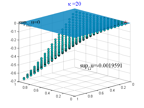
Figure 8 illustrates the numerical solutions and their maximum values on the domain boundary for the test problem (57) on the uniform square partitions of size 16×1616\times 16. The plots indicate that the maximum value of the numerical solution is not attained on the domain boundary, but satisfies the discrete maximum principle of max(x,y)Ωhubmax(x,y)Ωhmax(ub,0)\max_{(x,y)\in\Omega_{h}}u_{b}\leq\max_{(x,y)\in\partial\Omega_{h}}\max(u_{b},0) for all three cases of κ=0.7\kappa=0.7, 4.04.0, and 20.020.0.

Refer to caption
Refer to caption
Refer to caption
Fig. 8: Plot of numerical solutions and their maximum values on the domain boundary arising from the SWG scheme (12) for the test problem (57), using the uniform rectangular partition of size 16×1616\times 16.

In summary, the discrete maximum principle is satisfied for all three test problems for the case of κ=0.7\kappa=0.7 and κ=4\kappa=4. The result is in good consistency with the DMP theory developed in Theorem 2. The computational result also indicates a satisfaction of the DMP for the case of κ=20\kappa=20 for which no theory was known.

6.2 Numerical results for the finite difference scheme

The goal of this section is to investigate the performance of the finite difference scheme (12). For simplicity, we consider the model problem (1)-(2) with α=1\alpha=1, 𝜷=0{\bm{\beta}}=0, and c=0c=0 on the unit square domain Ω=(0,1)2\Omega=(0,1)^{2}. The two test cases in our numerical experiments assume the following exact solution and the right-hand side function:

{u=x(x1)y(y1),f=2x(x1)+2y(y1),\displaystyle\left\{\begin{array}[]{lllll}u=-x(x-1)y(y-1),\\ f=2x(x-1)+2y(y-1),\end{array}\right.
{u=sin(x)sin(y)x2+y2,f=2sin(x)sin(y).\displaystyle\left\{\begin{array}[]{lllll}u=-\sin(x)\sin(y)-x^{2}+y^{2},\\ f=-2\sin(x)\sin(y).\end{array}\right.

It is easy to see that the function ff is non-positve in both tests.

Table 4 show the error and convergence performance of the finite difference scheme (12). Optimal order of convergence can be seen for the L2L^{2} error, while a superconvergence of order 𝒪(h2){\mathcal{O}}(h^{2}) is illustrated for the numerical solution in the discrete H1H^{1} norm.

Table 4: Error and convergence performance of the finite difference scheme (12) for the test cases (6.2) and (6.2).
Test case (6.2), κ=4.0\kappa=4.0 Test case (6.2), κ=4.0\kappa=4.0
h1h^{-1} uhu0,h\|u_{h}-u\|_{0,h} r=r= uhu1,h\|u_{h}-u\|_{1,h} r=r= uhu0,h\|u_{h}-u\|_{0,h} r=r= uhu1,h\|u_{h}-u\|_{1,h} r=r=
8 4.59e-04 - 1.46e-03 - 3.47e-05 - 4.10e-04 -
16 1.14e-04 2.0 3.66e-04 2.0 8.63e-06 2.0 1.02e-04 2.0
32 2.85e-05 2.0 9.15e-05 2.0 2.15e-06 2.0 2.56e-05 2.0
64 7.12e-06 2.0 2.29e-05 2.0 5.33e-07 2.0 6.42e-06 2.0
128 1.78e-06 2.0 5.72e-06 2.0 1.30e-07 2.0 1.61e-06 2.0

Tables 5-6 show max(x,y)Ωhub(x,y)\displaystyle\max_{(x,y)\in\Omega_{h}}u_{b}(x,y) and max(x,y)Ωhub(x,y)\displaystyle\max_{(x,y)\in\partial\Omega_{h}}u_{b}(x,y) for the numerical solutions arising from the finite difference scheme (43). Table 5 is concerned with the case of the scheme with κ=0.7\kappa=0.7 and κ=4\kappa=4 for which the DMP theory is applicable. It can be seen from the table that max(x,y)Ωhub(x,y)<max(x,y)Ωhub(x,y)\displaystyle\max_{(x,y)\in\Omega_{h}}u_{b}(x,y)<\max_{(x,y)\in\partial\Omega_{h}}u_{b}(x,y) so that the (strong) DMP is verified. For curiosity, we also tested the case of κ=20\kappa=20 for which no DMP theory is known. It is interesting to note that the discrete maximum principle still holds true for the case of κ=20\kappa=20, as shown in Table 6.

We point out that a penalization method was employed to implement the Dirichlet boundary condition in our computation so that the numerical boundary values are slightly different from the exact boundary data.

Table 5: DMP verification of the finite difference scheme (43) for the test problem (6.2) with κ=0.7\kappa=0.7 and κ=4\kappa=4 on uniform partitions.
Test problem (6.2)
κ=0.7\kappa=0.7 κ=4.0\kappa=4.0
hh 1/8 1/32 1/128 1/8 1/32 1/128
maxΩub(x,y)\displaystyle\max_{\partial\Omega}u_{b}(x,y) -7.5e-11 -4.9e-12 -2.4e-13 -6.5e-11 -4.6e-12 -3.0e-13
maxΩub(x,y)\displaystyle\max_{\Omega}u_{b}(x,y) -7.5e-03 -4.9e-04 -3.0e-05 -6.5e-03 -4.6e-04 -3.0e-05
Test problem (6.2)
κ=0.7\kappa=0.7 κ=4.0\kappa=4.0
hh 1/8 1/32 1/128 1/8 1/32 1/128
maxxΩub(x,y)\displaystyle\max^{~}_{x\in\partial\Omega}u_{b}(x,y) 0.9435 0.9866 0.9966 0.9435 0.9866 0.9966
maxxΩub(x,y)\displaystyle\max_{x\in\Omega}u_{b}(x,y) 0.7448 0.9408 0.9855 0.7627 0.9419 0.9855
Table 6: DMP verification of the finite difference scheme (43) for the test problems (6.2) and (6.2) with κ=20.0\kappa=20.0 on uniform meshes.
Test problem (6.2), κ=20.0\kappa=20.0 Test problem (6.2), κ=20.0\kappa=20.0
hh 1/8 1/32 1/128 1/8 1/32 1/128
maxΩub(x,y)\displaystyle\max_{\partial\Omega}u_{b}(x,y) -6.3e-11 -4.6e-12 -3.0e-13 0.9435 0.9866 0.9966
maxΩub(x,y)\displaystyle\max_{\Omega}u_{b}(x,y) -6.3e-03 -4.6e-04 -3.0e-05 0.7682 0.9423 0.9856
Refer to caption
Refer to caption
Refer to caption
Fig. 9: DMP verification of the finite difference scheme (43) for the test problem (6.2), using the uniform partition of size 32×3232\times 32.

References

  • [1] E. Bertolazzi and G. Manzini, A second-order maximum principle preserving finite volume method for steady convection-diffusion problems, SIAM J. Numer. Anal., 43, pp. 2172-2199, 2005.
  • [2] A.J. Christlieb, Y. Liu, Q. Tang, and Z. Xu, High order parametrized maximum-principle-preserving and positivity-preserving WENO schemes on unstructured meshes, J. Comput. Phys., 281, pp. 334-351, 2015.
  • [3] P.G. Ciarlet, The Finite Element Method for Elliptic Problems, Classics Appl. Math. 40, SIAM, Philadelphia, 2002.
  • [4] P. Ciarlet and P.-A. Raviart, Maximum principle and uniform convergence for the finite element method, Comput. Methods Appl. Mech. Eng., 2, pp. 17-31, 1973.
  • [5] J. Droniou and C.L. Potier, Construction and convergence study of schemes preserving the elliptic local maximum principle, SIAM J. Numer. Anal., 49, pp. 459-490, 2011.
  • [6] A. Drăgănescu, T.F. Dupont, and L.R. Scott, Failure of the discrete maximum principle for an elliptic finite element problem, Math. Comput., 74, pp. 1-24, 2004.
  • [7] L. Evans, Partial Differential Equations, vol. 19 of Graduate Studies in Mathematics, American Mathematical Society, Providence, Rhode Island, 2010.
  • [8] V. Girault and P.-A. Raviart, Finite Element Methods for the Navier-Stokes Equations: Theory and Algorithms, Springer-Verlag, Berlin, 1986.
  • [9] W. Huang, Y. Wang, Discrete maximum principle for the weak Galerkin method for anisotropic diffusion problems, Commun. Comput. Phys., 18, pp. 65-90, 2015.
  • [10] D. Li, C. Wang, and J. Wang, Superconvergence of the gradient approximation for weak Galerkin finite element methods on nonuniform rectangular partitions, https://arxiv.org/pdf/1804.03998v2.pdf.
  • [11] Q. Li and J. Wang, Weak Galerkin finite element methods for parabolic equations, Numer. Methods Partial Differ. Equ., 29, pp. 1-21, 2013.
  • [12] Y. Liu and J. Wang, Simplified Weak Galerkin and Finite Difference Schemes for the Stokes Equation[J], arXiv preprint arXiv:1803.00120, 2018.
  • [13] Y. Liu and J. Wang, A simplified weak Galerkin finite element method: algorithm and error estimates, arXiv:1808.08667v2, 2018.
  • [14] L. Mu, J. Wang, G. Wei, X. Ye, and S. Zhao, Weak Galerkin methods for second order elliptic interface problems, J. Comput. Phys., 250, pp. 106-125, 2013.
  • [15] L. Mu, J. Wang, and X. Ye, A weak Galerkin finite element method with polynomial reduction, Journal of Computational and Applied Mathematics, vol. 285, pp. 45-58, 2015.
  • [16] M.K. Mudunuru and K.B. Nakshatrala, On enforcing maximum principles and achieving element-wise species balance for advection-dffusion-reaction equations under the finite element method, Journal of Computational Physics, Volume 305, 15, pp. 448–493, 2016.
  • [17] G. Strang and G.J. Fix, An Analysis of the Finite Element Method, Prentice Hall, Englewood Cliffs, NJ, 1973.
  • [18] R.S. Varga, On a discrete maximum principle, SIAM J. Numer. Anal., 3, pp. 355-359, 1966.
  • [19] C. Wang and J. Wang, A primal-dual weak Galerkin finite element method for second order elliptic equations in non-divergence form, Math. Comp., vol. 87, 515-545, 2018. DOI: https://doi.org/10.1090/mcom/3220. June 2017.
  • [20] J. Wang and X. Ye, A weak Galerkin mixed finite element method for second-order ellliptic problems. arXiv: 1104.2897vl. J. Comp. and Appl. Math., 241, 103-115, 2013.
  • [21] J. Wang and X. Ye. A weak Galerkin mixed finite element method for second-order elliptic problems, Math. Comp., 83, pp. 2101-2126, 2014.
  • [22] J. Wang, X. Ye, Q. Zhai, and R. Zhang, Discrete maximum principle for the P1P_{1}-P0P_{0} weak Galerkin finite element approximations, J. Comput. Phys., 362, pp. 114-130, 2018.
  • [23] J. Wang and R. Zhang, Maximum principles for P1-conforming finite element approximations of quasi-linear second order elliptic equations, SIAM J. Numer. Anal., 50, pp. 626-642, 2012.
  • [24] Y. Zhang, X. Zhang, and C.-W. Shu, Maximum-principle-satisfying second order discontinuous Galerkin schemes for convection-diffusion equations on triangular meshes, J. Comput. Phys., 234, pp. 295-316, 2013.