

Unsupervised anomaly localization in high-resolution breast scans using deep pluralistic image completion
Abstract
Automated tumor detection in Digital Breast Tomosynthesis (DBT) is a difficult task due to natural tumor rarity, breast tissue variability, and high resolution. Given the scarcity of abnormal images and the abundance of normal images for this problem, an anomaly detection/localization approach could be well-suited. However, most anomaly localization research in machine learning focuses on non-medical datasets, and we find that these methods fall short when adapted to medical imaging datasets. The problem is alleviated when we solve the task from the image completion perspective, in which the presence of anomalies can be indicated by a discrepancy between the original appearance and its auto-completion conditioned on the surroundings. However, there are often many valid normal completions given the same surroundings, especially in the DBT dataset, making this evaluation criterion less precise. To address such an issue, we consider pluralistic image completion by exploring the distribution of possible completions instead of generating fixed predictions. This is achieved through our novel application of spatial dropout on the completion network during inference time only, which requires no additional training cost and is effective at generating diverse completions. We further propose minimum completion distance (MCD), a new metric for detecting anomalies, thanks to these stochastic completions. We provide theoretical as well as empirical support for the superiority over existing methods of using the proposed method for anomaly localization. On the DBT dataset, our model outperforms other state-of-the-art methods by at least 10% AUROC for pixel-level detection.
1 Introduction
Anomaly detection (AD) refers to the task of detecting patterns in data that are not present in normal data. It is an important and safety-critical task in medical imaging and many other fields. In many situations, little or no anomalous data is available, making it crucial to develop methods that can perform AD using only normal data for training, a task known as unsupervised anomaly detection Bergmann et al. 2019. This is because traditional supervised computer vision models requires large amounts of both normal and anomalous data for training, making them not applicable to this scenario. This research direction is especially important in the medical imaging field where it is often resource-intensive to acquire new data. Such methods are referred to as unsupervised or self-supervised learning methods.
In this manuscript, we consider the realistic case of Digital Breast Tomosynthesis (DBT) data, a relatively new breast cancer screening modality that has gained traction in recent years. It is difficult to develop AD methods for these images, due to the high rarity of cancer cases and the natural anatomical variability seen in both healthy and cancerous cases. The high resolution of DBT poses an additional challenge for tumor detection methods because the images cannot always be downsampled to a lower resolution without losing the fine-grained anatomical detail present in breast tissue that may be necessary for accurate tumor detection.
Indeed, we find that standard deep learning-based AD methods, which perform well on non medical-image domains, have poor performance on DBT scans. Deep methods are vulnerable to (1) the high visual similarity of certain normal and cancerous DBT images that leads to images of different classes appearing very similar, and (2) the aforementioned high resolution problem, which are both issues that are less present in the natural image datasets that standard deep AD methods are evaluated on (e.g., Bergmann et al. 2019). This motivates our advanced unsupervised image anomaly detection method, which solves the problem from a different perspective.
An intuitive way of thinking about an anomalous image is that the content in the image is unexpected, given knowledge of what normal data looks like. This intuition can be implemented in the unsupervised or self-supervised regime, as it does not require any explicit knowledge about anomalous data. In particular, we solved this problem through image completion beginning with our earlier work of Swiecicki et al. 2021, i.e., if some region of an image is removed and a completion network is asked to “fill in” a normal prediction given the surroundings, and the predicted region and the original region are different, then that region can be considered anomalous.
However, a shortcoming of this approach is that the output completion, despite being realistic, is fixed for a given input. False positives can occur if only a single possible (deterministic) normal completion is predicted by the network, given that there can be various valid completions for a region. Many masked images theoretically have a multimodal distribution of possible completions, so a completely anomaly-free ground truth region could be distinctively different from the completion that the network happens to output. In other words, any dissimilarity of the original image to just one of the possible predictions is an imprecise measure of abnormality. Moreover, the presence of multiple valid completions is especially prominent in data with high semantic variability, such as breast tissue scans.
To remedy this problem, our approach uses a pluralistic image completion network to sample from the distribution of possible normal completions to compare to the ground truth, which we achieve using a novel and simple application of spatial (channel-wise) dropout layers to a pretrained image completion network. Even if certain surroundings of a normal ground truth have a high number of semantically distinct valid normal completions, we are guaranteed to eventually sample a completion that is similar to the ground truth, provided that the pluralistic network is a strong approximation of the true distribution of valid normal completions. However, if the ground truth is anomalous, then it is very unlikely that any valid normal completion is similar to it, because the two samples are from fundamentally distinct distributions.
Following this observation, we expect that given a large sample of normal completions, if the ground truth is normal, the distance of the closest completion to the ground truth will be greater if the ground truth is anomalous than if it is normal. We can quantify this idea by taking the minimum of all of the distances from each completion to the ground truth, and hypothesizing that this minimum distance will generally be greater for anomalous ground truths than for normal ground truths. From these ideas we propose a new anomaly score metric: minimum completion distance, or MCD. We have shown both theoretically and empirically that it is a more faithful measure of abnormality.
Given a 2D slice of a pseudo-3D DBT scan volume, our method works by sampling multiple completions of successive patches on a “sliding” raster window on the slice/image. We can detect anomalies within the spatial location of each patch using our MCD metric, which analyzes how similar the ground truth of the completion region is to the sampled completions; if the ground truth is sufficiently different from the sampled completions, we assume that the region contains an anomaly. This procedure is performed on many overlapping patches that cover the entire image, so that a full anomaly heatmap can be generated at the end using the spatially-oriented anomaly scores of each patch. We perform patch-level anomaly detections in parallel, along both the number of completions to sample per patch, and the number of patches to complete. Our overall method is named PICARD, or Pluralistic Image Completion for Anomalous Representation Detection. We provide Python/PyTorch code for our method at https://github.com/mazurowski-lab/picard.
Novel Contributions
In summary, our contributions are the following:
- 1.
We introduce a novel anomaly localization model that uses channel-wise dropout on image patches to rapidly sample pluralistic completions of patches in order to localize anomalies on the image.
- 2.
We propose a novel evaluation metric, MCD, for completion similarity assessment and anomaly scoring. We provide a thorough analysis of the effectiveness of this metric.
- 3.
By adopting existing state-of-the-art methods that aim for natural / low-resolution images, we build an anomaly localization performance benchmark on the challenging DBT dataset, in which our method outperforms these methods by a large margin. This benchmark also serves as a foundation for future works.
The rest of this manuscript is organized as follows: In Section 2, we explore related works. In Section 3 we mathematically analyze the effectiveness of MCD, and our method used to achieve pluralistic image completion. In Sections 4 and 5 we present our target dataset and experimental results, respectively. Finally, in Section 6 we discuss our findings and outline future research directions, and in Section 7 we summarize our conclusions.
2 Related Works
Anomaly Localization with Self-Supervised Learning
The tasks of anomaly detection (AD), i.e., the classification of entire images as being either normal or anomalous, and anomaly localization/segmentation (AL), i.e., the spatial segmentation of anomalies within images, have received considerable attention within the fields of machine learning and deep learning in particular. Many AD works exist Choi et al. 2018; Ren et al. 2019; Grathwohl et al. 2019; Nalisnick et al. 2018; Nalisnick et al. 2019; Serrà et al. 2019; Du and Mordatch 2019; Schlegl et al. 2019; Choi and Chung 2019; Deecke et al. 2018; Pidhorskyi et al. 2018, but we consider AL, the more challenging task that is also more applicable to clinical practice.
The vast majority of AL methods benchmark on the industrial anomaly detection dataset MVTec-AD Bergmann et al. 2019. Recent works include CutPaste, a self-supervised learning model which trains an encoder neural network to extract features that are useful for differentiating between normal and anomalous data on the proxy task of detecting the “cutting and pasting” of regions of images to another random part of the image Li et al. 2021; PatchSVDD, a patch-based self-supervised model that utilizes support vector data descriptions (SVDDs) to detect and localize anomalies Yi and Yoon 2020; PatchCore, which localizes anomalies within patches by comparing their features to a memory bank of features of patches from normal images based on pretrained neural networks Roth et al. 2021; and PaDiM, a similar patch-based method that estimates the probability distribution of normal class instances Defard et al. 2020. These methods detect anomalies by comparing image features to features from normal training data; our method instead compares directly to a normal “realization” of the image given its surroundings, which is more robust to the high complexity of medical data, in particular breast tissue, where the possible feature similarity between anomalous and normal data can be much higher as compared to other types of data such as MVTec-AD. This is one possible reason for why these other methods, which perform very well on MVTec-AD, have a performance drop on medical data such as DBT, while our method performs significantly better.
Although MVTec-AD serves to model the application of anomaly localization to the industrial setting, the task of AL for medical images is also an important task for multiple reasons. First, we find that AL methods that perform extremely well on MVTec-AD do not necessarily translate well to medical image AL scenarios. This is due to the MVTec-AD data being significantly more controlled, less complex, and much less varied than the data seen in medical images, as well as having visual similarities to images from ImageNet, which have been absorbed by commonly-used pretrained image encoders, i.e., ResNet He et al. 2016. Healthy tissue in medical images often has high semantic variability, uncountably many distinct possible anomalies, and can generally be quite unpredictable, especially in highly variable anatomies like the breast. Simply put, many existing AL methods do not have the ability to fully generalize to the many possible challenging scenarios of medical anomaly detection. We believe that supporting a greater focus of general AD and AL research on the important, safety-critical application of medical imaging is essential for the development of methods that have broader impact.
Anomaly Localization with Image Completion
Another direction of AL is to reconstruct a test image and consider it as anomalous if the reconstruction is distinct from the input. Reconstruction-based methods, e.g., Schlegl et al. 2019; Choi and Chung 2019; Deecke et al. 2018; Pidhorskyi et al. 2018, commonly solve this problem through an encoder-decoder mechanism. These methods can not always be robust at discriminating anomalous data from normal data because given some input image, anomalous data within it may be partially reconstructed even by a normal-trained reconstructor, making anomalies not stand out within the reconstruction error. Image completion-based methods, e.g., Haselmann et al. 2018; Munawar and Creusot 2015; Pirnay and Chai 2021b; Zavrtanik et al. 2021; Pirnay and Chai 2021a; Swiecicki et al. 2021, alleviate this problem by excluding the reconstructed region as input, and creating a normal completion that is more noticeably different than the anomalous ground truth.
Recent works Wan et al. 2021; Liu et al. 2021a; Zhao et al. 2020; Zheng et al. 2019; Dupont and Suresha 2019 approached the goal of producing multiple plausible and diverse completions for a single input. As such, these methods are unnecessary and impractical for our purposes, which we show experimentally in Section 5.2.
Instead, we achieve completion variability by a simple and novel application of spatial dropout layers to a pretrained completion network. Our method requires no additional training, and could theoretically be used on any sort of convolutional deterministic completion network. This keeps our overall anomaly detection method straightforward and intuitive, and importantly, fast.
3 Methods
3.1 Introduction
Our overall anomaly localization method is summarized in Figures 1 (outer, image/slice-level loop) and 2 (inner, patch-level loop). Beginning with some 2D slice of a DBT scan volume, our model creates a “sliding” patch window that rasters through the slice with a fixed stride. For each sliding-window image patch , we apply a mask over the center region to obtain an image with the region missing; we save the missing region as the ground truth completion. Next we compare the distribution of predicted normal completions of to the ground truth completion , by examining the distance, in a feature space, of the prediction closest to the ground truth. If that distance is above a certain threshold, then is anomalous. In Figure 2, and are the feature space distributions of (1) anomalous and (2) normal completions of , respectively. The anomaly score for each is used for the associated locations of the anomaly heatmap of the entire DBT slice (Fig. 1).


3.2 The MCD Anomaly Metric and its Convergence Properties
In this section we present the formal definition of the minimum completion distance (MCD) metric, which we use for anomaly detection at the patch level. Anomaly localization is then performed for an entire DBT slice by using the MCD metric on overlapping patches of that slice.
Consider a single test image/patch with a ground truth completion region that has surroundings , i.e., and . Now, consider sampling i.i.d. (independent and identically distributed) possible normal completions of : . Here is the probability density function (p.d.f.) of the distribution of possible normal completions of ; we denote as the same but for anomalous completions.
Now, use a pretrained normal data encoder to map the completions to a feature space via . Assuming to be an injective function, we can construct p.d.f.s of completions within this feature space; i.e., the feature space p.d.f. paired with is . As such, transforms the completion image samples to .
We then define the MCD anomaly score of to be
| (1) |
where is the ground truth completion in feature space.
Next, we show that this metric is an arbitrarily powerful anomaly classifier as the sample size approaches , and more practically that the performance improves with high sample efficiency, given reasonable assumptions about how the distributions of anomalous and normal data are distanced from each other. These assumptions are adapted from Proposition 2 of Ye et al. 2021, and are summarized as follows:
Key Assumptions Appropriate for Anomaly Detection
Given any test image with completion region and surroundings , the feature-space distributions of possible normal and anomalous completions of , and , respectively, are sufficiently distant such that for most , is small enough so that almost everywhere (see the dashed-line box at the bottom left of Fig. 2).
The AUROC/AUC, or Area Under the Receiver Operating Characteristic Curve, is a widely-used method for quantifying the performance of a classifier. One way of defining it is that the AUC is the probability of a positive sample being given a score higher than a negative sample Fawcett 2006; Yuan et al. 2020. Consider some patch with completion region and surroundings that has no anomalies within , and some other patch with completion region and surroundings that does have anomalies within . In this case, the definition of the AUC translates to the probability that the patch with an anomalous completion region will be scored higher than the patch with a normal completion region, i.e., . To optimize our anomaly metric for a given patch, we would like to maximize this equation. Next, we will evaluate the asymptotic performance of our novel metric’s AUC with respect to , in order to provide a formal analysis of our method’s performance.
Convergence Derivation
To begin, for readability we will define the minimum distance anomaly scores of and respectively as and via Equation (1). Note that are i.i.d. random variables. The normal ground truth can also be thought of as being sampled from because it is just another valid completion of ; similar reasoning applies to the anomalous ground truth and . As such, and are both continuous random variables (as both are functions of continuous random variables). We then have
| (2) | ||||
| (3) |
where the second line was obtained because and are independent, as they are respectively generated from possible completions of independent images.
The inner integral is the cumulative density function of evaluated at some given ,
| (4) | ||||
| (5) |
Now, is the probability that out of the sample , there is no for such that , i.e. . This probability can therefore be computed as
| (6) | ||||
| (7) | ||||
| (8) | ||||
| (9) | ||||
| (10) | ||||
| (11) |
where the product expansion can be taken because each feature space completion sample of is independent. The term within the product is the probability that the feature space distance between the (fixed) ground truth of the completion region and the (random) possible normal completion sample is less than the given . This is found by integrating the probability density of normal completions (in feature space) that all of the were sampled from, , over the “-ball” with centered at , defined by .
This integral can be written as
| (12) |
allowing Eq. (11) to become
| (13) |
as the integral is the same for all samples of possible normal completions of the masked image , because it only depends on and , the latter of which is computed with samples from the distribution of normal completions of the other masked image .
As such, Equation (5) can be written as
| (14) |
which can be substituted into Eq. (3) to give
| (15) | ||||
| (16) | ||||
| (17) |
written with an expectation value as
| (18) |
Recall that our goal is to evaluate the limit of the MCD metric AUC (Eq. (18)) with respect to the normal completion sample size . Note that the normal completion probability density integral term within the expectation, , is bounded by for all because is bounded by , as is a zero probability event where a sampled is exactly . This means that is also bounded by , and therefore so is , which means that the expectation of Eq. (18) is as well. As for all , then it must be the case that , so that
| (19) | ||||
| (20) |
i.e. the classifier theoretically approaches a perfect AUC as the sample size . We evaluate this behavior empirically in Section 5.3.
However, for practical purposes we must consider how this score performs for a reasonably-sized ; from Eq. (18) we need to be sufficiently close to zero for a low enough .
We can achieve a better empirical performance guarantee by applying the previously stated assumptions of anomaly detection. First note that as increases, will continually decrease, as remains the same or decreases as . A useful AUC for a satisfactorily-low will occur if the term decreases quickly as increases. In fact, our earlier work of Swiecicki et al. 2021 is built on the case of . Through our spatial dropout method that we use for pluralistic completions (Section 3.3), our method can generate any unique completions, thus allowing for a higher AUC.
By assumption, the normal and anomalous distributions and , respectively, are sufficiently distant that it is unlikely that samples from one will be close to samples from the other. Now, consider steadily incrementing from . For an anomalous , will begin large, and although likely getting slightly smaller as increases due to additional samples, it is expected to stay reasonably large, making decrease quickly. Even if some sample happens to be close to , any sampling where this is non-trivially likely to happen will have high enough for to already be very small despite the accompanying low , so this is a non-issue. It is also very unlikely for to begin small, although this would be a “failure mode” as would only decrease slowly from there. In summary, we should achieve good performance for a low ; indeed we find in practice that is sufficient to achieve beyond state-of-the-art anomaly localization results, and the influence of different choices of is shown in Section 5.3 as well.
3.3 Completion Variability with Spatial Dropout
We have shown theoretical support for our MCD anomaly metric, and explained why given appropriate assumptions of the distributions of normal and anomalous data, the metric performs well for a reasonably small completion sample size . The central component of this metric is the diverse sampling from : the distribution of possible normal completions of some surroundings ; in other words, obtaining pluralistic completions. We opt for a simple and intuitive approach for creating pluralistic completions that still manages to achieve sufficient feature variability of completions for the MCD metric. Our goal is to make the output of a completion network trained on normal data variable for some fixed input masked image . At each evaluation of we wish to obtain a different output completion , while still maintaining the ability of to create fairly realistic normal inpaintings that will be distinct from any anomalous data.
Our intuition is from the dropout Srivastava et al. 2014 mechanism, which is commonly used during training to combat overfitting, but can also be used during inference to produce variable outputs Kendall and Gal 2017. We apply this general prescription to a completion network to induce variability for conditional generative models. This idea is briefly introduced in Wieluch and Schwenker 2019, but they only present it as a proof-of-concept extension of their work, while we manage to implement it in a real application setting.
In particular, we perform completions using the model of Yu et al. 2018, which includes a Wasserstein generative adversarial network (GAN)-based fully-convolutional completion network and critic/encoder Arjovsky et al. 2017. creates a fixed completion of some input masked image , while learns to discriminate between real vs. fake normal completion data; we use as the completion feature encoder described in Section 3.2. Wasserstein generative adversarial networks (GANs) are signicantly more reliable to train than traditional GANs Goodfellow et al. 2014: they converge reliably, remove problems such as mode collapse, and have interpretable loss functions, among other benefits. The critic is the Wasserstein GAN’s version of the traditional GAN’s discriminator.
In our setting, since the input to is , a fixed variable, the network has no inherent stochasticity by default. A simple method of adding stochasticity to the input, i.e., where is sampled from some noise distribution, would not work as well because the network would simply learn to ignore Isola et al. 2017; Mathieu et al. 2015. In order to allow to create semantically diverse yet sufficiently high-quality completions at each evaluation of a single , we propose using spatial, or channel-wise dropout Tompson et al. 2015 within . This type of dropout randomly makes entire channels of convolutional layer activation maps zero with some probability, rather than individual neurons. We give examples of pluralistic completions using our method in Figure 3. We note that using dropout on naturally results in reduced visual quality of individual completions, due to the variability that dropout adds to the network. However, we found that the benefit of having access to multiple possible completions outweighs this, still resulting in improved tumor detection performance over the single-completion case (Table 2).
Conceptually, because convolutional layer activation maps carry spatial correlations between adjacent pixels, dropping out individual activations randomly can result in low-quality completions, which we found to be the case in practice. On the other hand, dropping an entire channel of an activation map with spatial dropout, can be thought of as inducing a change in the global feature information of the resulting completion, while avoiding any such negative spatial effects. This makes intuitive sense at a high level: for a given layer of a fully connected neural network, the individual neuron’s activations are the key global features that affect the downstream inference; on the other hand, for a convolutional neural network layer, the key global features are different channels of the given activation map. Lee and Lee 2020 in fact found that spatial dropout used on convolutional neural networks (CNNs) can be functionally similar to using regular dropout on fully connected neural networks.

Intriguingly, we did not find any benefit in the quality or diversity of pluralistic completions between the options of (1) using dropout on during both training and testing or (2) only testing, over the course of many experiments. As such, for the sake of simplicity, we obtain pluralistic completions by only applying dropout at test time to a normally (non-dropout) trained completion network. We also obtained better inpainting quality (on the training set) when dropout is excluded from the shallowest and deepest layers of (see Appendix A.1 for details). For all experiments we use a dropout probability of , a relatively high value that we found suitable for generating sufficiently diverse completions, which was also assisted by dropout being used after the majority of ’s layers. We found that different training iterations of sometimes resulted in differing quality and variability of completions once dropout was applied, but we saw no obvious trends to this, so chose to halt training simply when the distance between completions and ground truth was minimized (see Section 5.1 for more training details).
It is also conceivable to explicitly optimize the placement and probabilities of dropout layers to maximize completion diversity and visual quality. However, there is not an explicit, differentiable dependence of a completion diversity metric (e.g., LPIPS Zhang et al. 2018) or quality metric (e.g., the critic/discriminator score) on the dropout layer parameter(s) and/or placement, so it is unclear how these parameters could be efficiently tuned to optimize for these metrics. Doing so would require a non-differentiable optimization method such as Bayesian optimization, which is computationally prohibitive due to the high number of possible dropout parameters to tune (layer-by-layer), and the computational cost of sampling enough completions at each iteration of such a routine to get a reasonable holistic measure of completion diversity and quality. We attempted this Bayesian optimization procedure in early experiments but found that it did not converge; due to these issues, we simply fixed the dropout probability to a fixed value (0.5) for all layers, which we found sufficient for completion diversity and quality.
Our method also has the added benefit that only negligible additional computational load is needed to create a pluralistic completion compared to an ordinary deterministic completion network, as each completion is created by an independent forward pass through . This also makes pluralistic completion sampling easily parallelizable.
3.4 Full Anomaly Localization Method: PICARD
We can now determine whether some patch of a DBT scan includes an anomaly within the center square region by sampling possible normal completions of that region given the surroundings, and using the minimum completion distance (MCD) metric (Eq. (1)) to compare the completions to the missing region ground truth. The final portion of our model is to use this new metric to localize, or segment, anomalies within a full size DBT slice.
Anomaly localization requires synthesizing an anomaly heatmap for a given DBT slice that is the same size as that slice, where each pixel of the heatmap corresponds to the model’s prediction confidence of the corresponding slice pixel containing anomalous data. To do so, we begin with the image patch at the top left of —our “window”—and apply the MCD metric to that patch, with the aforementioned masked region chosen a priori, to obtain an anomaly score associated with that patch. We then shift the window by some stride according to a basic overlapping raster scan order, perform the same procedure to obtain an anomaly score for this next window, and repeat until all raster windows have been scored, ending with the patch at the bottom right of . The heatmap is all of these scores arranged with the same spatial orientation of the corresponding raster patch centers that created the scores. Finally, we use bicubic interpolation to upsample the heatmap until it is of the same size as . The overall anomaly localization procedure is summarized in Algorithm 1. In practice, the two for loops are parallelized to take full advantage of GPU memory; i.e., multiple completions are sampled, for multiple inputs, all at once. This feature creates a large decrease in computation time compared to our previous work of Swiecicki et al. 2021, where completions were simply made one-at-a-time.
Input: Input DBT scan , patch size , mask size , pluralistic completion sample size , and completion network with completion encoder/critic , both pretrained on normal data.
4 Dataset
For all experiments we use full size 2D slices of breast cancer DBT Digital Breast Tomosynthesis (DBT) scans from the Breast Cancer Screening (BCS)-DBT dataset Buda et al. 2021. The scans have resolutions of either or pixels. For training all models we used healthy slices of DBT volumes from the training set of BCS-DBT, each of which come from a different anatomical view and/or patient. -shaped patches are randomly sampled from these slices for pretraining the completion network and the encoder for PICARD. For testing we use DBT slices that each contain at least one radiologist-annotated tumor, obtained from the test set of BCS-DBT. The tumor bounding-box annotations in the test set range in size from about to of the total area of a DBT image. All DBT slices are left-aligned for symmetry. We provide more details for the creation of this dataset and the impact of using it to test anomaly localization in Appendix C. Code for reproducing all experiments will be made publicly available.
| Dataset | No. of DBT scan slices |
| Training (healthy only) | 6,245 |
| Testing (biopsied cancer only) | 133 |
5 Experiments and Results
Given that the outputs from our method are pixel-wise heatmaps, and only ground truth lesion bounding boxes are provided in BCS-DBT, we adopt pixel AUC/AUROC as our anomaly localization (AL) evaluation metric, as in other AL works Schlegl et al. 2019; Yi and Yoon 2020; Roth et al. 2021; Li et al. 2021; Defard et al. 2020. We note that such AL algorithms cannot be evaluated with object-level detection metrics such as IoU because they do not output binary localization predictions such as segmentations or bounding boxes, as tuning some method used to seperate the heatmap into foreground and background pixels and then form object boxes/masks would require a validation set containing labeled anomalies, which is not permissible within the AL/AD setting.
Specifically, we label all pixels of the slice as negative, except for the pixels inside and along the bounding box(es), which we label as positive. To obtain an anomaly localization/pixel AUC score for a given image, each pixel’s binary label (normal or anomalous) is compared to the corresponding anomaly score from our model’s predicted heatmap for that pixel, and the pixel is classified as anomalous if its score is above a certain threshold. The pixel-wise AUC for the image analyzes all possible score thresholds for a given image/heatmap to provide a holistic measure of anomaly localization performance for the entire image. The final performance metric for the entire test set is the average pixel AUC of all slices. We also include a specific example of the associated ROC curve with the anomaly score distributions of normal and anomalous pixels created by using PICARD to heatmap a DBT slice from the test set in Figure 4.
5.1 DBT Tumor Localization
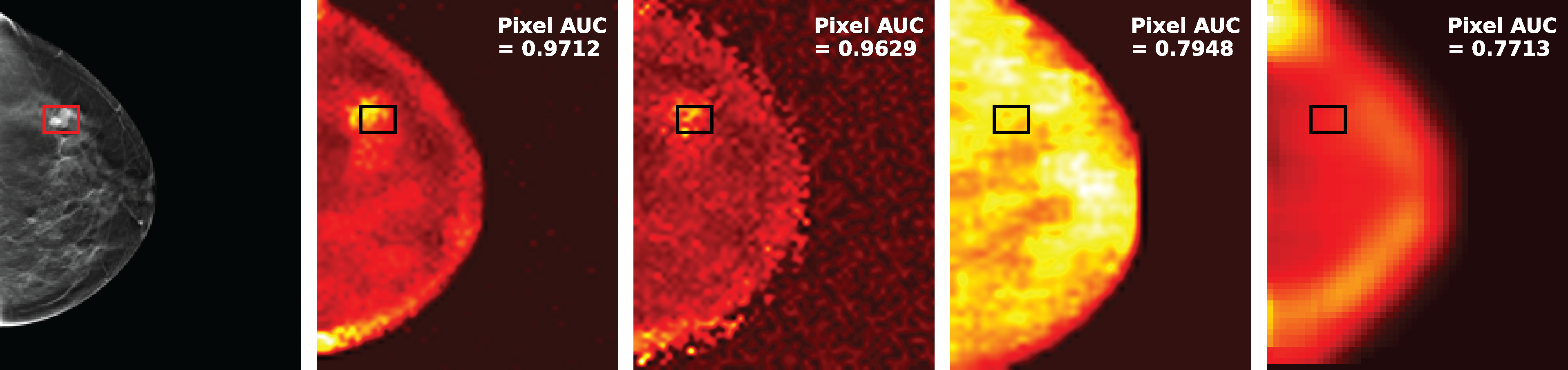
Now we compare previous leading unsupervised/self-supervised anomaly localization methods to our work: quantitative (pixel AUC) results are summarized in Table 2, while qualitative (anomaly heatmap) results are given in Figure 5. We also provide the pixel-wise average precision (AP) score for each method in Table 2. The AP summarizes the precision-recall curve, and is the weighted mean of the precision achieved at each possible scoring threshold along the precision-recall curve, according to scikit-learn’s sklearn.metrics.average_precision_score in Python. Further details and results of these comparison studies are given as follows, where we first explore other state-of-the-art methods, followed by our model.
| Method | Pixel AUC | Pixel AP |
| ||
|
0.875 | 0.0943 | 0.062 | ||
|
0.865 | 0.0672 | 0.064 | ||
|
0.846 | 0.0817 | 0.062 | ||
|
0.826 | 0.0582 | 0.064 | ||
| PatchSVDD Yi and Yoon 2020 | 0.777 | 0.0303 | 4.13 | ||
| CutPaste Li et al. 2021 | 0.737 | 0.0522 | 0.087 |




CutPaste Li et al. 2021
CutPaste first learns self-supervised deep representations and then builds a generative one-class classifier on learned representations. The representations are learned by classifying normal data from a novel data augmentation strategy that cuts an image patch and pastes it at a random location of a large image. To localize defective regions, CutPaste crops the images before applying the augmentation. CutPaste obtained leading anomaly localization results on the most common benchmark of MVTec-AD Bergmann et al. 2019.
To make a fair comparison to our method, we adopt the best performing augmentation strategy (CutPaste 3-Way) and use the sliding-window hyperparameters as for PICARD. We further adjust the method to not select blank image patches or paste them in blank regions. These changes increase the classification difficulty and improve the performance. We train CutPaste until loss convergence, at epochs.
During inference, we extract embeddings from all patches with a given stride and learn a generative classifier at each location via a simple parametric Gaussian density estimator (GDE), with a log-probability density of , where specifics the spatial location for the current image patch , and is the feature embedding network. The final anomaly score map is obtained by accumulating prediction scores from all the generative classifiers. We find that CutPaste obtains an anomaly localization result on the DBT test set of average pixel AUC. A few example heatmaps are shown in Figure 5.
PatchSVDD Yi and Yoon 2020
PatchSVDD is an extension of DeepSVDD Ruff et al. 2018 to solve the problem of high-level intra-class variations by adopting patches, instead of entire images, as network inputs. It alleviates the collapse issue of mapping features to a single center by minimizing the distances between features extracted from spatially adjacent patches. The method also proposes an additional self-supervised learning task to predict the relative location of two nearby patches.
Since this method also makes the predictions at patch level, we can directly adopt this method in our setting. To make it compatible with the DBT dataset, we select the same patch and stride size as PICARD, and , respectively. During inference, we also use the same protocol PatchSVDD proposed to generate the anomaly map for every DBT image. We follow the same training parameters and procedure as in the original paper, and set the loss scaling hyperparameter . On the DBT test set, PatchSVDD achieves pixel AUC. Several example heatmaps are presented in Figure 5.
PICARD (ours)
Lastly, we evaluate our method, PICARD, (Figs. 1, 2 and Algorithm 1), on the DBT test dataset. We set patch size and mask size . Empirically, this setting is sufficient enough to allow room for high resolution, variable completions to capture a variety of anomalies, while small enough to be able to precisely localization anomalies on the much larger, global DBT slices, which have resolutions of approximately . For all experiments we set the raster window stride to pixels (so that the raster windows overlap), and we set completion sample size . We trained the inpainter and critic with a batch size of , halting once the training set reconstruction error between completions and their corresponding ground-truth images stopped decreasing. All experiments were completed on four 24 GB NVIDIA RTX 3090 GPUs. Each heatmap took approximately two minutes to create, by processing multiple sliding raster window inputs, each sampling multiple completions, all in parallel. All other experimental and model training details are given in Appendix A.1.
On the test set, PICARD achieves an average pixel-level AUC for lesion detection of with the MCD metric in image space, and in feature space, outperforming other existing methods by at least AUC. We find that when we set in order to evaluate the single completion case, these values shift to and for image and feature space, respectively. These are the first BCS-DBT pixel AUC results for this method that was first introduced in our work of Swiecicki et al. 2021, which itself already beats other state-of-the-art methods. We also find that our approach similarly outperforms all other methods in average precision. Of note is that our model requires no hyperparameter optimization on some validation set, ensuring that it can be trained and prepared for use only using healthy data.
Breast tumors can greatly vary in size between cases (Section 4), so it is important that our model can detect both very small and very large tumors. We see in the case shown in the right top row of Fig. 5 that our method is able to localize an extremely small tumor, while other methods fail to do so. In the opposite case of a very large tumor shown in the right second row of the same figure, our model is also able to localize the tumor and make it stand out compared to the surrounding tissue area, despite the tumor being much larger than the size of the raster window/patch. This is a very important property of our method, as it allows for the localization of tumors of a wide range of sizes.
We also note our model’s performance on cases with dense breast tissue, shown in the bottom row of Fig. 5, where the surrounding tissue of the tumor is visually similar to the tumor itself. As the tumor is not easily distinguishable from the surrounding tissue, this is a challenging case for both anomaly localization algorithms and radiologists Nazari and Mukherjee 2018. However, our method is still able to localize the tumors in this case, while the other existing approaches both fail to differentiate it from its surroundings.
Finally, we also evaluate the inference speed of our approach compared to existing methods, per image patch, shown in the rightmost column of Table 2. We show that our method is about faster than CutPaste (0.062 sec. vs. 0.087 sec. per patch), and over faster than PatchSVDD (4.13 sec. per patch), while still possessing superior tumor detection performance. The large difference in inference speed between our method and PatchSVDD is due to the fact that PatchSVDD requires computing the distance of the patch’s features to every single image’s features in the training set, while our approach simply compares the patch’s features to the features of the completions of the patch (in parallel).
5.2 Using State-of-the-Art Pluralistic Image Completion Backbones
As few research considers the topic of pluralistic image completion, we compare our dropout pluralistic completion method (Section 3.3) to the state-of-the-art method of Wan et al. 2021, which presents a two-stage, transformer-based model for pluralistic image completion. We trained this method on the same random normal DBT patch dataset as the dropout inpainter, and example inpaintings created by the trained model are shown in Figure 3. Although the completions are slightly more detailed (but still not anatomically valid) than our dropout inpainter, in practice we find that this method is significantly slower than the dropout method for creating multiple completions, such that it becomes impractical for anomaly localization.
On a single 24 GB RTX 3090 GPU, it takes 2.9 days for HFPIC and 8 minutes for our method to generate a single heatmap with the default setting of an completion sample size. This difference is simply due to the significant margin between the size of the two models: ours has about million trainable parameters, while HFPIC has about million. We further evaluated this difference by (1) fixing , the number of input patches to complete, and testing a range of for both inpainting methods, and (2) fixing and testing a range of . The computation time results are shown in Figure 6; each datapoint was averaged over six possible input DBT slice patches from the test set. We see that in general, HFPIC is slower than our method by about three orders of magnitude.
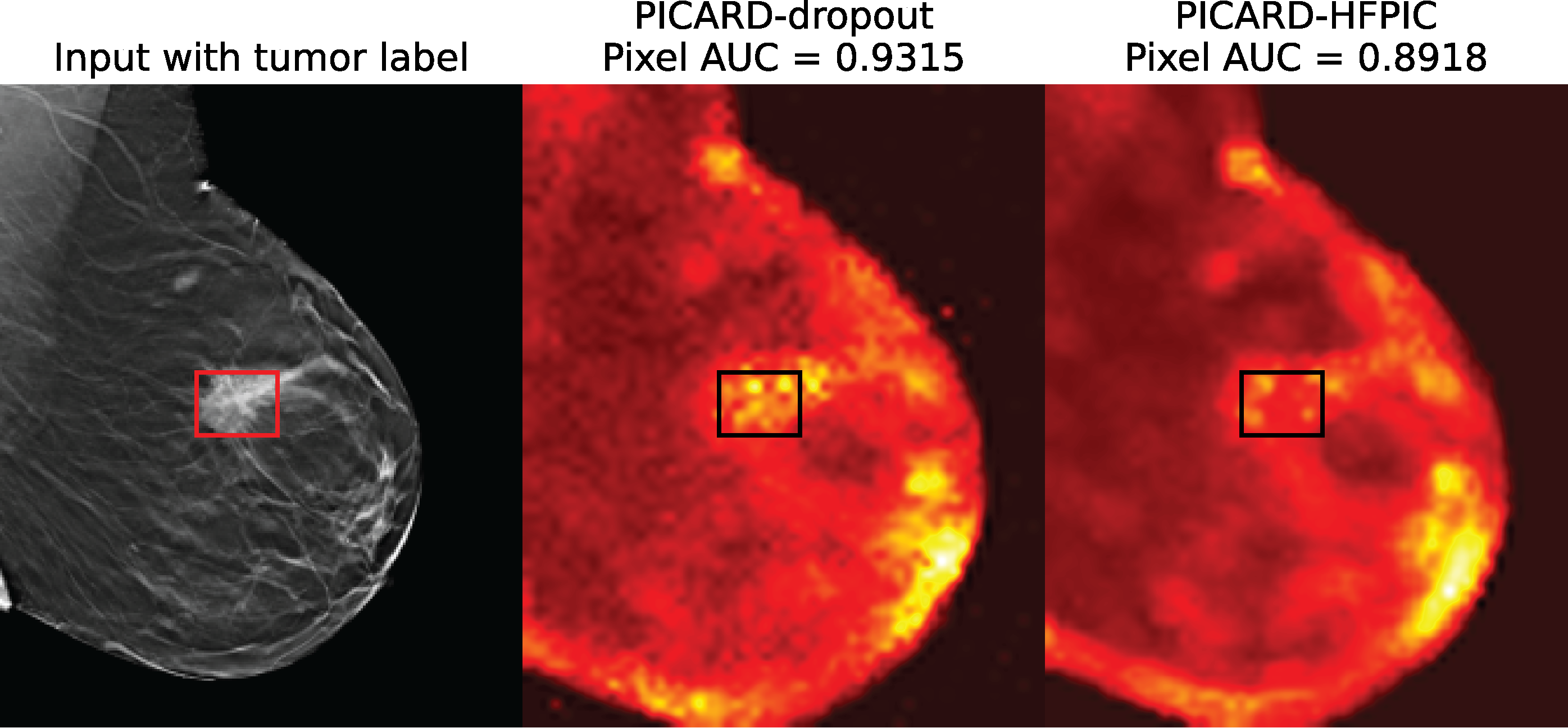
Moreover, we have tested the effectiveness of HFPIC by using it to create a heatmap for a DBT slice in the test set. Although the extreme computation time makes it impractical to test PICARD with HFPIC on the entire test set, we tested it on a single image (which took days to compute) shown in Figure 7. Here, we actually see a decrease in anomaly localization performance; this is likely due to the anatomically unrealistic nature of HFPIC DBT completions, as shown in Figure 3.
5.3 Asymptotic Behavior of the MCD Metric
In Section 3.2 we showed that theoretically, the MCD metric (Equation 1) achieves perfect AUC performance in the limit of inpainting sample size . We evaluate this behavior empirically in order to validate these claims by calculating the tumor localization performance (pixel AUC) of PICARD on a range of values of , , on a set of ten DBT scans randomly sampled from the test set, shown in Figure 8. We use a subset instead of the full testing set due to computation feasibility (it takes almost 6 days to evaluate the entire set with ). Performance does indeed increase asymptotically as , but not to a perfect AUC of . This is due to the fact that in our derivations, we assume that the pluralistic inpainter is able to perfectly sample from the true distribution of possible completions; in practice, the inpainting method is necessarily imperfect, as it is difficult to capture the broad anatomical variability and complexity of breast tissue. Finally, we note that this analysis was completed after all other experiments, where was chosen a priori.
6 Discussion
The central result of this work is that our pluralistic image completion-based anomaly localization (AL) method performs much better on DBT data than existing AL methods Li et al. 2021; Yi and Yoon 2020 that have been shown to perform well on common machine learning AL benchmarks like MVTec-AD Bergmann et al. 2019. Importantly, these existing works differ from our approach in that they all rely on directly comparing the features of the input image to some learned distribution of normal features, not to new normal (inpainting) features that are created by our model, and conditioned on the same surroundings as the input completion region. This fundamental difference in how anomaly localization/detection is approached is one reason for the superiority of our method. The MVTec-AD benchmark that the other methods do well with has normal data that vary minimally within a single object class, anomalous data that fall into one of several, in fact labeled cases, and normal and anomalous data that have starkly different, and easily separable, features. These characteristics make anomaly detection easier, in terms of feature discrimination and generalization. However, DBT data does not possess these properties; healthy and cancer breast tissue possesses extreme semantic variability, and in many cases anomalous tissue can appear quite similar to healthy tissue (and vice versa). As such, it stands to reason that these existing methods generalize poorly when extended to DBT. We believe that this is excellent evidence for utilizing the BCS-DBT dataset as a new benchmark for anomaly detection research in machine learning, due to the life-critical application yet high complexity of the data, and the fact that it is publicly available.
While DBT tumor localization serves as a challenging benchmark for our anomaly localization algorithm, our approach is designed from a general standpoint, such that a wider range of applications are possible. As such, an important direction of future research is to extend our method to anomaly localization scenarios in other biomedical imaging modalities. These could include modalities such as OCT (optical coherence tomography), MRI (magnetic resonance imaging) or others.
Interestingly, converting completions to the encoder feature space for PICARD did not introduce any performance boost as opposed to other AL methods; we hypothesize that this is again because breast tissue data is more complex and difficult to grasp useful features from than the natural image data that many of these other methods are built for. As we have already achieved strong performance with the current model, we leave it to future works to develop a feature encoder that could possibly be more robust to this type of data. Indeed, this could be related to the poor performance of the other, feature-discriminating AL methods, that do much better with natural or industrial images that have easier features to work with.
6.1 Limitations
The superior results of PICARD for DBT breast lesion detection are quite promising, however, further refinements could be applied to make the method even more powerful.
One of the difficulties of generative modeling of breast tissue is the extremely high complexity and natural variability of the tissue, so that it is difficult to obtain anatomically realistic completions, even with state-of-the-art methods like HFPIC Wan et al. 2021. In addition to complex local details, breast tissue can have complicated correlations between distant image locations, which may not be able to be fully captured by the inherent locality of convolutional neural networks models. Indeed, the coarse-to-fine feature hierarchy of traditional convolutional image completion methods–such as the one used in this work–is well-suited for natural images, where low-resolution features are more global, yet it is unable to fully represent the complexities of breast tissue. Visual transformer-based models, e.g., Dosovitskiy et al. 2020; Liu et al. 2021b can model long-range pixel interactions, but even the transformer-based model of HFPIC was unable to produce anatomically realistic content. As such, it is unclear what type of generative model would be able to learn reasonable representations of breast data that preserve both local fine-grained details while maintaining the complex global structure of the tissue. Such a model may need to include some sort of inductive biases for the unique structures seen in visual anatomical data; alternatively, entirely different generative models may prove useful, such as normalizing flows, energy-based, or score-based methods, which we leave for future works.
Having more realistic completions would better approximate sampling from the true distribution of possible completions, theoretically leading to more robust minimum completion distance performance, and therefore better anomaly localization. This would fix some of the issues of false-positive regions that can be seen in some of PICARD’s heatmaps, that have breast tissue that is labeled as healthy, but still possesses visual features that are uncommon in the training set. We found that even training our inpainter(s) on the full DBT training set of normal slices did not improve performance, so it appears to be a limitation of the model structure rather than the dataset size.
Although PICARD’s tumor localization performance does receive a boost from using multiple completions instead of just one (present in the first two rows of Table 2 where , vs. the next two with ), in theory the difference could be higher, again if the sampled completions were more realistic and better approximated the true distribution of possible normal completions. One possible solution to this would be to choose a dropout probability for the completion network that results in optimal anatomical realism. However, such optimization needs access to some cancer images during the validation phase, greatly reducing its range of applications. It may be possible to quantify the anatomical realism of completions generated on some validation set of only healthy cases, and optimize the dropout probability to maximize this quantity, but we leave this nontrivial task for future works.
Another possible future work is that as the completion region is our region of interest, we made no assumptions about if the surrounding region contains anomalies. Still, it may be worth considering how to detect anomalies within as well, which could begun with considering the joint distribution rather than just as in this work. However, it is unclear if this would improve heatmapping performance, as we use a stride small enough such that all pixels (beyond a “padding region” on the border) within a DBT slice will be included at least once within some evaluated .
7 Conclusion
We introduced a novel anomaly localization method for ultra-high-resolution DBT breast scan data, called PICARD. We found that PICARD achieves promising performance with this difficult modality, that existing methods in the machine learning literature struggle to match. PICARD compares a distribution of pluralistic normal image completions to the ground truth, and uses a new lightweight and efficient way to sample pluralistic completions using spatial dropout layers on a pretrained completion network. We also introduced a formal foundation for completion-based anomaly detection, and used it to mathematically analyze the convergence properties of our anomaly score. Finally, we synthesized all of these contributions into the final PICARD method.
Acknowledgments
We would like to thank Jichen Yang and Brian Harrawood at Duke University for assisting with dataset downloading and management.
Funding
This work was supported by Grant 1 R01 EB021360 from the National Institutes of Health (PI: Mazurowski).
References
- Arjovsky et al. (2017) Martin Arjovsky, Soumith Chintala, and Léon Bottou. Wasserstein generative adversarial networks. In International conference on machine learning, pages 214–223. PMLR, 2017.
- Bergmann et al. (2019) Paul Bergmann, Michael Fauser, David Sattlegger, and Carsten Steger. Mvtec ad–a comprehensive real-world dataset for unsupervised anomaly detection. In Proceedings of the IEEE/CVF Conference on Computer Vision and Pattern Recognition, pages 9592–9600, 2019.
- Buda et al. (2020) Mateusz Buda, Ashirbani Saha, Ruth Walsh, Sujata Ghate, Nianyi Li, Albert Swiecicki, Joseph Y Lo, and Maciej A Mazurowski. Detection of masses and architectural distortions in digital breast tomosynthesis: a publicly available dataset of 5,060 patients and a deep learning model. arXiv preprint arXiv:2011.07995, 2020.
- Buda et al. (2021) Mateusz Buda, Ashirbani Saha, Ruth Walsh, Sujata Ghate, Nianyi Li, Albert Swiecicki, Joseph Y Lo, and Maciej A Mazurowski. A data set and deep learning algorithm for the detection of masses and architectural distortions in digital breast tomosynthesis images. JAMA network open, 4(8):e2119100–e2119100, 2021.
- Choi et al. (2018) Hyunsun Choi, Eric Jang, and Alexander A Alemi. Waic, but why? generative ensembles for robust anomaly detection. arXiv preprint arXiv:1810.01392, 2018.
- Choi and Chung (2019) Sungik Choi and Sae-Young Chung. Novelty detection via blurring. arXiv preprint arXiv:1911.11943, 2019.
- Deecke et al. (2018) Lucas Deecke, Robert Vandermeulen, Lukas Ruff, Stephan Mandt, and Marius Kloft. Image anomaly detection with generative adversarial networks. In Joint european conference on machine learning and knowledge discovery in databases, pages 3–17. Springer, 2018.
- Defard et al. (2020) Thomas Defard, Aleksandr Setkov, Angelique Loesch, and Romaric Audigier. Padim: a patch distribution modeling framework for anomaly detection and localization. arXiv preprint arXiv:2011.08785, 2020.
- Dosovitskiy et al. (2020) Alexey Dosovitskiy, Lucas Beyer, Alexander Kolesnikov, Dirk Weissenborn, Xiaohua Zhai, Thomas Unterthiner, Mostafa Dehghani, Matthias Minderer, Georg Heigold, Sylvain Gelly, et al. An image is worth 16x16 words: Transformers for image recognition at scale. arXiv preprint arXiv:2010.11929, 2020.
- Du and Mordatch (2019) Yilun Du and Igor Mordatch. Implicit generation and modeling with energy based models. 2019.
- Dupont and Suresha (2019) Emilien Dupont and Suhas Suresha. Probabilistic semantic inpainting with pixel constrained cnns. In The 22nd International Conference on Artificial Intelligence and Statistics, pages 2261–2270. PMLR, 2019.
- Elson et al. (2007) Jeremy Elson, John R Douceur, Jon Howell, and Jared Saul. Asirra: a captcha that exploits interest-aligned manual image categorization. CCS, 7:366–374, 2007.
- Fawcett (2006) Tom Fawcett. An introduction to roc analysis. Pattern recognition letters, 27(8):861–874, 2006.
- Goodfellow et al. (2014) Ian Goodfellow, Jean Pouget-Abadie, Mehdi Mirza, Bing Xu, David Warde-Farley, Sherjil Ozair, Aaron Courville, and Yoshua Bengio. Generative adversarial nets. In Advances in neural information processing systems, pages 2672–2680, 2014.
- Grathwohl et al. (2019) Will Grathwohl, Kuan-Chieh Wang, Jörn-Henrik Jacobsen, David Duvenaud, Mohammad Norouzi, and Kevin Swersky. Your classifier is secretly an energy based model and you should treat it like one. arXiv preprint arXiv:1912.03263, 2019.
- Haselmann et al. (2018) Matthias Haselmann, Dieter P Gruber, and Paul Tabatabai. Anomaly detection using deep learning based image completion. In 2018 17th IEEE International Conference on Machine Learning and Applications (ICMLA), pages 1237–1242. IEEE, 2018.
- He et al. (2016) Kaiming He, Xiangyu Zhang, Shaoqing Ren, and Jian Sun. Deep residual learning for image recognition. In Proceedings of the IEEE conference on computer vision and pattern recognition, pages 770–778, 2016.
- Howlader et al. (1975) Nea Howlader, AM Noone, M Krapcho, J Garshell, D Miller, SF Altekruse, CL Kosary, M Yu, J Ruhl, Z Tatalovich, et al. Seer cancer statistics review. National Cancer Institute, 2008, 1975.
- Isola et al. (2017) Phillip Isola, Jun-Yan Zhu, Tinghui Zhou, and Alexei A Efros. Image-to-image translation with conditional adversarial networks. In Proceedings of the IEEE conference on computer vision and pattern recognition, pages 1125–1134, 2017.
- Kendall and Gal (2017) Alex Kendall and Yarin Gal. What uncertainties do we need in bayesian deep learning for computer vision? arXiv preprint arXiv:1703.04977, 2017.
- Krizhevsky et al. (2009) Alex Krizhevsky, Geoffrey Hinton, et al. Learning multiple layers of features from tiny images. 2009.
- Lee and Lee (2020) Sanghun Lee and Chulhee Lee. Revisiting spatial dropout for regularizing convolutional neural networks. Multimedia Tools and Applications, 79(45):34195–34207, 2020.
- Lehman et al. (2017) Constance D Lehman, Robert F Arao, Brian L Sprague, Janie M Lee, Diana SM Buist, Karla Kerlikowske, Louise M Henderson, Tracy Onega, Anna NA Tosteson, Garth H Rauscher, et al. National performance benchmarks for modern screening digital mammography: update from the breast cancer surveillance consortium. Radiology, 283(1):49–58, 2017.
- Li et al. (2021) Chun-Liang Li, Kihyuk Sohn, Jinsung Yoon, and Tomas Pfister. Cutpaste: Self-supervised learning for anomaly detection and localization. In Proceedings of the IEEE/CVF Conference on Computer Vision and Pattern Recognition, pages 9664–9674, 2021.
- Li et al. (2020) Ke Li, Gang Wan, Gong Cheng, Liqiu Meng, and Junwei Han. Object detection in optical remote sensing images: A survey and a new benchmark. ISPRS Journal of Photogrammetry and Remote Sensing, 159:296–307, 2020.
- Liu et al. (2021a) Hongyu Liu, Ziyu Wan, Wei Huang, Yibing Song, Xintong Han, and Jing Liao. Pd-gan: Probabilistic diverse gan for image inpainting. In Proceedings of the IEEE/CVF Conference on Computer Vision and Pattern Recognition, pages 9371–9381, 2021a.
- Liu et al. (2021b) Ze Liu, Yutong Lin, Yue Cao, Han Hu, Yixuan Wei, Zheng Zhang, Stephen Lin, and Baining Guo. Swin transformer: Hierarchical vision transformer using shifted windows. arXiv preprint arXiv:2103.14030, 2021b.
- Mathieu et al. (2015) Michael Mathieu, Camille Couprie, and Yann LeCun. Deep multi-scale video prediction beyond mean square error. arXiv preprint arXiv:1511.05440, 2015.
- Munawar and Creusot (2015) Asim Munawar and Clement Creusot. Structural inpainting of road patches for anomaly detection. In 2015 14th IAPR International Conference on Machine Vision Applications (MVA), pages 41–44. IEEE, 2015.
- Nalisnick et al. (2018) Eric Nalisnick, Akihiro Matsukawa, Yee Whye Teh, Dilan Gorur, and Balaji Lakshminarayanan. Do deep generative models know what they don’t know? arXiv preprint arXiv:1810.09136, 2018.
- Nalisnick et al. (2019) Eric Nalisnick, Akihiro Matsukawa, Yee Whye Teh, and Balaji Lakshminarayanan. Detecting out-of-distribution inputs to deep generative models using typicality. arXiv preprint arXiv:1906.02994, 2019.
- Nazari and Mukherjee (2018) Shayan Shaghayeq Nazari and Pinku Mukherjee. An overview of mammographic density and its association with breast cancer. Breast cancer, 25(3):259–267, 2018.
- Nilsback and Zisserman (2008) Maria-Elena Nilsback and Andrew Zisserman. Automated flower classification over a large number of classes. In 2008 Sixth Indian Conference on Computer Vision, Graphics & Image Processing, pages 722–729. IEEE, 2008.
- Pidhorskyi et al. (2018) Stanislav Pidhorskyi, Ranya Almohsen, Donald A Adjeroh, and Gianfranco Doretto. Generative probabilistic novelty detection with adversarial autoencoders. arXiv preprint arXiv:1807.02588, 2018.
- Pirnay and Chai (2021a) Jonathan Pirnay and Keng Chai. Inpainting transformer for anomaly detection. arXiv preprint arXiv:2104.13897, 2021a.
- Pirnay and Chai (2021b) Jonathan Pirnay and Keng Chai. Inpainting transformer for anomaly detection. arXiv preprint arXiv:2104.13897, 2021b.
- Ren et al. (2019) Jie Ren, Peter J Liu, Emily Fertig, Jasper Snoek, Ryan Poplin, Mark A DePristo, Joshua V Dillon, and Balaji Lakshminarayanan. Likelihood ratios for out-of-distribution detection. arXiv preprint arXiv:1906.02845, 2019.
- Roth et al. (2021) Karsten Roth, Latha Pemula, Joaquin Zepeda, Bernhard Schölkopf, Thomas Brox, and Peter Gehler. Towards total recall in industrial anomaly detection. arXiv preprint arXiv:2106.08265, 2021.
- Ruff et al. (2018) Lukas Ruff, Robert A. Vandermeulen, Nico Görnitz, Lucas Deecke, Shoaib A. Siddiqui, Alexander Binder, Emmanuel Müller, and Marius Kloft. Deep one-class classification. In Proceedings of the 35th International Conference on Machine Learning, pages 4393–4402, 2018.
- Russakovsky et al. (2015) Olga Russakovsky, Jia Deng, Hao Su, Jonathan Krause, Sanjeev Satheesh, Sean Ma, Zhiheng Huang, Andrej Karpathy, Aditya Khosla, Michael Bernstein, et al. Imagenet large scale visual recognition challenge. International journal of computer vision, 115(3):211–252, 2015.
- Schlegl et al. (2019) Thomas Schlegl, Philipp Seeböck, Sebastian M Waldstein, Georg Langs, and Ursula Schmidt-Erfurth. f-anogan: Fast unsupervised anomaly detection with generative adversarial networks. Medical image analysis, 54:30–44, 2019.
- Serrà et al. (2019) Joan Serrà, David Álvarez, Vicenç Gómez, Olga Slizovskaia, José F Núñez, and Jordi Luque. Input complexity and out-of-distribution detection with likelihood-based generative models. arXiv preprint arXiv:1909.11480, 2019.
- Srivastava et al. (2014) Nitish Srivastava, Geoffrey Hinton, Alex Krizhevsky, Ilya Sutskever, and Ruslan Salakhutdinov. Dropout: a simple way to prevent neural networks from overfitting. The journal of machine learning research, 15(1):1929–1958, 2014.
- Swiecicki et al. (2021) Albert Swiecicki, Nicholas Konz, Mateusz Buda, and Maciej A Mazurowski. A generative adversarial network-based abnormality detection using only normal images for model training with application to digital breast tomosynthesis. Scientific reports, 11(1):1–13, 2021.
- Tompson et al. (2015) Jonathan Tompson, Ross Goroshin, Arjun Jain, Yann LeCun, and Christoph Bregler. Efficient object localization using convolutional networks. In Proceedings of the IEEE conference on computer vision and pattern recognition, pages 648–656, 2015.
- Wah et al. (2011) Catherine Wah, Steve Branson, Peter Welinder, Pietro Perona, and Serge Belongie. The caltech-ucsd birds-200-2011 dataset. 2011.
- Wan et al. (2021) Ziyu Wan, Jingbo Zhang, Dongdong Chen, and Jing Liao. High-fidelity pluralistic image completion with transformers. arXiv preprint arXiv:2103.14031, 2021.
- Wieluch and Schwenker (2019) Sabine Wieluch and Friedhelm Schwenker. Dropout induced noise for co-creative gan systems. In Proceedings of the IEEE/CVF International Conference on Computer Vision Workshops, pages 0–0, 2019.
- Xiao et al. (2017) Han Xiao, Kashif Rasul, and Roland Vollgraf. Fashion-mnist: a novel image dataset for benchmarking machine learning algorithms. arXiv preprint arXiv:1708.07747, 2017.
- Ye et al. (2021) Fei Ye, Huangjie Zheng, Chaoqin Huang, and Ya Zhang. Deep unsupervised image anomaly detection: An information theoretic framework. In 2021 IEEE International Conference on Image Processing (ICIP), pages 1609–1613. IEEE, 2021.
- Yi and Yoon (2020) Jihun Yi and Sungroh Yoon. Patch svdd: Patch-level svdd for anomaly detection and segmentation. In Proceedings of the Asian Conference on Computer Vision, 2020.
- Yu et al. (2018) Jiahui Yu, Zhe Lin, Jimei Yang, Xiaohui Shen, Xin Lu, and Thomas S Huang. Generative image completion with contextual attention. In Proceedings of the IEEE conference on computer vision and pattern recognition, pages 5505–5514, 2018.
- Yuan et al. (2020) Zhuoning Yuan, Yan Yan, Milan Sonka, and Tianbao Yang. Robust deep auc maximization: A new surrogate loss and empirical studies on medical image classification. arXiv preprint arXiv:2012.03173, 2020.
- Zavrtanik et al. (2021) Vitjan Zavrtanik, Matej Kristan, and Danijel Skočaj. Reconstruction by inpainting for visual anomaly detection. Pattern Recognition, 112:107706, 2021.
- Zhang et al. (2018) Richard Zhang, Phillip Isola, Alexei A Efros, Eli Shechtman, and Oliver Wang. The unreasonable effectiveness of deep features as a perceptual metric. In Proceedings of the IEEE conference on computer vision and pattern recognition, pages 586–595, 2018.
- Zhao et al. (2020) Lei Zhao, Qihang Mo, Sihuan Lin, Zhizhong Wang, Zhiwen Zuo, Haibo Chen, Wei Xing, and Dongming Lu. Uctgan: Diverse image inpainting based on unsupervised cross-space translation. In Proceedings of the IEEE/CVF Conference on Computer Vision and Pattern Recognition, pages 5741–5750, 2020.
- Zheng et al. (2019) Chuanxia Zheng, Tat-Jen Cham, and Jianfei Cai. Pluralistic image completion. In Proceedings of the IEEE/CVF Conference on Computer Vision and Pattern Recognition, pages 1438–1447, 2019.
- Zheng et al. (2018) Xin Zheng, Yong Wang, Guoyou Wang, and Jianguo Liu. Fast and robust segmentation of white blood cell images by self-supervised learning. Micron, 107:55–71, 2018.
Supplementary Material for “Unsupervised anomaly localization in high-resolution breast scans using deep pluralistic image completion”
Appendix A Implementational Details
We implemented all of our methods and experiments in PyTorch. For all experiments, we fix the random seed to make the work reproducible. In all scripts we used a seed of with the basic code shown below:
A.1 Network Architecture and Experimental Details for PICARD (Our Method)
When applying spatial dropout to the (convolutional) layers of , we also found it important to not just apply dropout to every single layer, but to exclude certain layers from dropout for better performance. In particular we found it essential to not apply dropout to the first or last convolutional layers of (conv1 and conv17) and (conv1 and allconv17), as not doing so can result in possible identical “noise” completions that are occasionally sampled with a frequency proportional to the dropout probability. For this particular completion network we also found that excluding dropout on all of the layers following the final atrous/dilated layer conv10_atrous improved the quality of completions. Specifically, we observed that if these layers are included for dropout, occasionally dark regions appeared in feature maps on this part of the network that seeded unrealistic regions in the final completion. We reason that this is because these post-atrous layers perform interpolation to upsample the feature maps to increase the resolution to the final output resolution, so that initially small artifacts may become much more problematic as data is passed through further layers.
To convert completions in image space to a useful feature space, we use the feature map output of the final convolutional layer (conv4) of the WGAN critic as our encoder , flattened to be in . We also note that this critic is actually the local critic in the original work of Yu et al. 2018, takes completion regions as inputs alone. This is opposed to the global critic, which takes entire completed images as inputs. We pretrained the completion network and critic/encoder on the DBT patch dataset using the default procedure and hyperparameters of Yu et al. 2018, with a batch size of . We trained until we saw the reconstruction error between the inpaintings and the ground truths get no lower, at 130,000 iterations, on two NVIDIA RTX 3090 24GB GPUs. We generated all PICARD heatmaps with four 3090 24GB GPUs.
We also experimented with only including pixels within the breast (not in the outside black region that is within each slice) for the AUC calculation/heatmapping procedure, but we decided that it would be best to include the entire image to have the least number of experimental biases as possible, and to observe the performance of all models in all parts of the slice.
A.2 Experimental Details for Other Methods
HFPIC Wan et al. 2021
Transformer/coarse prior generator training: We used the default setting that the HFPIC authors used for ImageNet Russakovsky et al. 2015, except trained from scratch on the BCS-DBT training set (Table 1). Specifically, we used the BERT training objective, the GELU_2 activation function, and randomly generated pconv completion masks. For the transformer, we used 35 layers, an embedding size of 1024, and 8 heads. We trained for 200 epochs on a batch size of 6.
Convolutional network/guided upsampler training: Just as for the transformer, we used the default setting that the HFPIC authors used for ImageNet, except trained from scratch on the BCS-DBT training set (Table 1). We trained with a batch size of for iterations, on randomly generated pconv completion masks.
We chose the best performing models from each of their training according to the paper’s original validation score on normal image patches. Inference was performed with the same parameters as in training. We performed all experiments on one 48 GB NVIDIA RTX A6000 GPU.
A.3 Computational Efficiency
Our heatmapping model enjoys high scalability, by allowing for both the computation of multiple completions for a given input, and the computation of multiple inputs, all at the same time. This was created using PyTorch’s inherent support for parallelism; the former is completed by inputting copies of the same input image to the image completion model as a single, parallelized batch, while the latter is completed by creating a custom data loader that can load batches of heatmap raster windows, to be analyzed all at once.
One heatmap for a full size () DBT image is generated in just two minutes by four RTX 3090 GPUs. This is achievable by virtue of the relative simplicity and lack of additional computational load created by our dropout-based multi-inpainting method.
Appendix B Ablation Studies
B.1 Mean or Median Completion Distance instead of Minimum
By default, our approach uses the minimum completion distance/MCD anomaly scoring metric (equation (1)). Here we compare the tumor detection performance of the MCD metric with anomaly metrics that use the mean or median distance of normal completion samples to the ground truth,
| (21) |
and
| (22) |
respectively. Evaluated on tumor detection for the DBT test set as in Section 5.1, we found that our MCD metric outperforms the mean and median metrics, as shown in Table 3.
| Anomaly Metric | Pixel AUC |
| Min. CD/MCD (image space) | 0.875 |
| Min. CD/MCD (feature space) | 0.865 |
| Mean CD (image space) | 0.863 |
| Mean CD (feature space) | 0.843 |
| Median CD (image space) | 0.867 |
| Median CD (feature space) | 0.846 |
B.2 Regular Dropout Instead of Spatial Dropout
In practice, we found that using regular dropout on can introduce pixelated artifacts within completions and/or significantly less plausible completions than for when we used spatial dropout.
Appendix C Dataset Details
In this paper we work with the BCS-DBT (Breast Cancer Screening-Digital Breast Tomosynthesis) dataset of ultra-high-resolution 3D breast cancer scans, originally from Buda et al. 2020 and recently published as Buda et al. 2021. This dataset is a collection of breast scans that are divided into four disjoint classes, of which we use normal (no potential lesions flagged by a radiologist), and cancer (contains lesion(s) flagged by a radiologist, biopsied and confirmed to be cancer). Each scan is a 3D volume of about 70 physically-adjacent 2D greyscale scan slices, where each slice is a image. For our training set we take healthy slices from the BCS-DBT training set, from different patients. Each slice is sampled randomly from a different anatomical view/volume, originating from different patients in total. For our test set, we take all slices from the BCS-DBT test set that have radiologist-annotated biopsied lesion(s) (as each lesion annotation corresponds to one of the slices, or in rare cases, multiple lesions per slice). The massive class imbalance is due to the rarity of breast cancer: for regular screening mammograms, only about of women obtain positive result for cancer Lehman et al. 2017.
The BCS-DBT dataset is useful for evaluating image anomaly detection methods for a number of reasons:
- 1.
It represents an important real-world application of anomaly detection: breast cancer detection, which is a leading cause of death in women. Approximately 1 in 8 women will be diagnosed with invasive breast cancer in their lifetime, and 1 in 39 women will die from it Howlader et al. 1975. On the other hand, many anomaly detection benchmarks seen in the general machine learning literature e.g., CIFAR-10 and CIFAR-100 do not clearly represent real-world anomaly detection use cases. The industrial anomaly dataset MVTec Bergmann et al. 2019 is an important exception to this, but it is still considerably simpler than medical anomaly datasets.
- 2.
The data is very high resolution, both normal and anomalous data have strong semantic variability within the two classes, and anomalous data can often appear similar to normal data, altogether forming a challenging dataset.
Furthermore, the dataset is specifically useful for our method because (1) there are an abundance of normal instances, which is necessary to train GAN based models, especially for high-resolution data; (2) there are radiologist-annotated bounding boxes that provide ground truths of cancerous lesions/anomalous data. Other anomaly detection benchmarks either do not possess bounding boxes for object instances, like CIFAR-10, CIFAR-100 Krizhevsky et al. 2009, FashionMNIST Xiao et al. 2017 and CatsVsDogs Elson et al. 2007, and/or do not have enough per-class instances to successfully train our GAN-based method on, such as 102 Category Flowers Nilsback and Zisserman 2008, Caltech UCSD Birds 200 Wah et al. 2011, MVTec Bergmann et al. 2019, WBC Zheng et al. 2018, or DIOR Li et al. 2020. The first criteria is important because our method is defined by the conditional information of the surroundings of the region of interest, which needs a bounding box that is known whether or not an anomalous object is within it. Still, in a future work we would like to attempt using a completion model that can be trained on low amounts of data, so that these datasets with relatively few per-class instances that do have anomaly/object bounding boxes, e.g., MVTec, could be tested on our method.
For our dropout inpainter, we pretrain the completion network and the critic/encoder on random patches of the training set. The network is trained to inpaint random rectangular masks of normal patches, while for testing, we always use centered square masks. We normalize all data to the range as used in Yu et al. 2018. We train the HFPIC inpainter on the same dataset of healthy scan patches.
The vast majority of the BCS-DBT dataset is publicly available (on https://wiki.cancerimagingarchive.net/pages/viewpage.action?pageId=64685580 ), except for a small portion, described as follows. The dataset is originally divided into a training set ( DBT scan volumes/DICOM files), a validation set () and a test set (). All raw image/DICOM files are public. Each of these sets have normal and cancer class instances, with two other classes that are not relevant for this work. The training set has a public list of both class labels for all scans, and lesion bounding boxes for cancerous scans.
However, the BCS-DBT validation and test sets do not currently include public labels and bounding boxes, which we plan to release soon.
Now, our method could still be trained and tested on the labeled data that IS publicly available, namely BCS-DBT’s training set. This training set contains total DBT volumes, a subset of which we used for training, and it contains 76 cancer scans that we did not use, that could be used for testing.