

GeoFUSE: A High-Efficiency Surrogate Model for Seawater Intrusion Prediction and Uncertainty Reduction
Abstract
Seawater intrusion into coastal aquifers poses a significant threat to groundwater resources, especially with rising sea levels due to climate change. Accurate modeling and uncertainty quantification of this process are crucial but are often hindered by the high computational costs of traditional numerical simulations. In this work, we develop GeoFUSE, a novel deep-learning-based surrogate framework that integrates the U-Net Fourier Neural Operator (U-FNO) with Principal Component Analysis (PCA) and Ensemble Smoother with Multiple Data Assimilation (ESMDA). GeoFUSE enables fast and efficient simulation of seawater intrusion while significantly reducing uncertainty in model predictions. We apply GeoFUSE to a 2D cross-section of the Beaver Creek tidal stream-floodplain system in Washington State. Using 1,500 geological realizations, we train the U-FNO surrogate model to approximate salinity distribution and accumulation. The U-FNO model successfully reduces the computational time from hours (using PFLOTRAN simulations) to seconds, achieving a speedup of approximately 360,000 times while maintaining high accuracy. By integrating measurement data from monitoring wells, the framework significantly reduces geological uncertainty and improves the predictive accuracy of the salinity distribution over a 20-year period. Our results demonstrate that GeoFUSE improves computational efficiency and provides a robust tool for real-time uncertainty quantification and decision making in groundwater management. Future work will extend GeoFUSE to 3D models and incorporate additional factors such as sea-level rise and extreme weather events, making it applicable to a broader range of coastal and subsurface flow systems.
Lawrence Berkeley National Laboratory
keypoints
A new deep-learning framework GeoFUSE is developed for rapid and accurate seawater intrusion simulations and data assimilation U-Net Fourier Neural Operator (U-FNO) acts as surrogate model to reduce simulation time from hours to seconds, achieve a speedup of 360,000 times An ensemble method, conditioned on observations, is used to reduce uncertainty in geomodels and flow predictionsPlain Language Summary
Seawater intrusion is an increasing threat to coastal areas due to climate change and rising sea levels. Predicting the movement of seawater through underground aquifers is essential for managing coastal water resources. However, traditional simulations are often slow, computationally expensive, and susceptible to inaccuracies due to uncertainty in geological systems. We developed a deep-learning-based framework, GeoFUSE, for rapid and accurate subsurface flow simulations that also reduces uncertainty by incorporating measurement data. Using a U-FNO surrogate model, we significantly accelerate the simulation process, while an ensemble method helps further reduce uncertainty in salinity distribution predictions. We demonstrate the effectiveness of the framework using the Beaver Creek tidal stream-floodplain system.
1 Introduction
Seawater intrusion into freshwater aquifers, driven by climate change and groundwater exploitation, has become an increasing threat to subsurface systems in coastal regions globally Werner et al. (2013); Ketabchi et al. (2016). The effects of seawater intrusion can be detrimental to both the environment and human activities, including contamination of freshwater and drinking water, disruption of ecosystems, impacts on agriculture, and damage to infrastructure. Efficient and accurate modeling of seawater intrusion is crucial for predicting the movement of the saltwater front and ensuring the sustainability of groundwater resources and ecosystems.
Researchers have applied multiple simulation techniques to address the growing threat of seawater intrusion and predict its impact on coastal aquifers. Tools such as SEAWAT Langevin & Guo (2006); Langevin et al. (2008), SUTRA Provost & Voss (2019), and PFLOTRAN Hammond et al. (2014); Yabusaki et al. (2020) are commonly used to simulate variable density groundwater flow and solute transport in both conceptual and real-site models. These simulations require a detailed parameterization of geology and aquifer properties, informed by both experiments and numerical modeling. Furthermore, model calibration and data assimilation are essential to improve predictive accuracy and reduce uncertainties. Typically, model calibration is conducted within a Bayesian framework, conditioned on monitoring data, and requires repeated simulations to quantify uncertainty Arora et al. (2011); Arora et al. (2012). However, forward simulations over long periods are computationally expensive, particularly when accounting for pressure changes caused by daily tidal effects. Furthermore, the inherent uncertainty of aquifer parameters in heterogeneous systems introduces significant variability into flow predictions. Despite advancements in modeling, these processes remain computationally intensive, and the requirement for numerous forward runs limits the efficiency of data assimilation. This work aims to reduce computational costs, enabling faster, more accurate predictions and mitigating uncertainty in geomodels and predictions.
To address computational challenges in subsurface applications, several traditional surrogate modeling techniques have been developed. These include artificial neural networks for multi-objective optimization Bhattacharjya & Datta (2009), genetic programming and modular neural networks Sreekanth & Datta (2010), Evolutionary Polynomial Regression Hussain et al. (2015), and Gaussian process emulators Rajabi & Ketabchi (2017). These models often focus on specific quantities within simulation-optimization schemes and may not effectively capture the temporal evolution of state variables, such as the spatial distribution of flow and salinity predictions, across entire simulation domains, particularly in geologically complex areas.
In contrast, recent deep learning approaches have shown significant potential in addressing the challenge of capturing the temporal evolution of state variables, particularly for spatio-temporal flow prediction in subsurface systems. For instance, Mo et al. (2019) developed deep autoregressive neural networks for predicting contamination transport, and Zhou & Tartakovsky (2021) used convolutional neural networks to identify contaminant sources. Other advancements include the recurrent residual U-net for two-phase flow problems Tang et al. (2020), which has been further adapted for multi-fidelity systems Jiang & Durlofsky (2023) and various geological scenarios Han et al. (2024). The Fourier Neural Operator (FNO) Li et al. (2020), designed to capture fluid dynamics in infinite-dimensional Fourier spaces, and the U-FNO, which combines FNO with a U-net architecture for improved accuracy and efficiency in geological carbon storage Wen et al. (2022), are notable innovations. U-FNO has been successfully applied to groundwater contamination problems, predicting flow responses under new parameter inputs and boundary conditions Meray et al. (2024). While U-FNO, with its strong ability to capture the temporal evolution of state variables, is particularly well-suited for seawater intrusion problems, it stands out for its efficiency in modeling complex interactions between saltwater and freshwater flows. This makes it a highly effective approach for generating accurate predictions under varying conditions, though other methods may also offer viable solutions depending on specific problem requirements and constraints.
To address the uncertainty inherent in heterogeneous subsurface geological systems, inverse modeling and data assimilation, widely applied in seawater intrusion studies, are essential for calibrating geological models based on monitoring data. For instance, Yoon et al. (2017) used pressure data with the Ensemble Kalman Filter (EnKF) to calibrate heterogeneous models for a saline aquifer, while Dodangeh et al. (2022) employed concentration measurements for joint inversion of contaminant sources and hydraulic conductivity in coastal aquifers. Similarly, Goebel et al. (2017) utilized Electrical Resistivity Tomography for inversion in Monterey’s coastal region, and Cao et al. (2024) proposed a deep-learning-based data assimilation method to infer non-Gaussian heterogeneous coastal aquifers. Recently, the Ensemble Smoother with Multiple Data Assimilation (ESMDA) method, developed by Emerick & Reynolds (2013), is a variant version of EnKF, has been widely applied to various subsurface flow problems, including contaminant transport Zhou et al. (2022) and geological carbon storage Jiang & Durlofsky (2024). The ESMDA method has demonstrated its ability to assimilate noisy and sparse measurements and can be extended to calibrate geological models for coastal systems. However, the computational costs of these inversion processes remain high, highlighting the need for integrating surrogate models to improve efficiency.
This work focuses on developing an efficient surrogate model to enable rapid seawater intrusion prediction and integrating it into a data assimilation framework for calibrating heterogeneous geological models. The ultimate goal is to reduce prediction uncertainty while improving computational efficiency. The framework is applied to a 2D cross-section of the Beaver Creek tidal stream-floodplain system Yabusaki et al. (2020), which serves as a representative case to assess the effects of tidal dynamics and the potential impacts of sea level rise on coastal systems.
The framework combines a surrogate model trained on PFLOTRAN-simulated data with a data assimilation process using Principal Component Analysis (PCA) and the ESMDA. This approach enables parameter reduction, model calibration, and uncertainty reduction in salinity predictions. By incorporating this method, we aim to significantly reduce computational costs while maintaining predictive accuracy, ultimately advancing subsurface modeling for more effective management of seawater intrusion in coastal environments.
2 Methodology
In this work, we apply U-Fourier neural operator (FNO) for rapid spatio-temporal flow predictions, while ESMDA is integrated conditioned on observational data to calibrate geological models, thereby reducing computational costs in seawater intrusion modeling and improving predictive accuracy for heterogeneous geological models. This combined framework, referred to as GeoFUSE (explained further in Section 2.3), is applied to a 2D cross-section of the Beaver Creek tidal stream-floodplain system Yabusaki et al. (2020). The U-FNO surrogate is trained on the simulation results of 2D multi-Gaussian permeability realizations.
The Beaver Creek model was developed by Yabusaki et al. (2020), who investigated the effects of tidal restoration on floodplain inundation and salinization by modeling subsurface flow and transport. Their study focused on the dynamics of a first-order tidal stream system, aiming to clarify the interactions between freshwater and seawater, as well as the processes controlling water levels and salinity in the floodplain. The Beaver Creek site is ideal for this study, as it improves our understanding of how tidal influences reshape hydrological and ecological patterns in restored environments. The complexities of tidal effects, salinization, and uncertain geological models make the problem computationally intensive. In the following sections, we describe the Beaver Creek model, surrogate model development, the GeoFUSE data assimilation framework, and performance evaluation in detail.
2.1 Beaver Creek Model and Governing Equations Using PFLOTRAN
The Beaver Creek model from Yabusaki et al. (2020) was developed using PFLOTRAN Hammond et al. (2014), a computational tool designed to simulate subsurface flow and reactive transport processes in variably saturated porous media. Given these capabilities, PFLOTRAN is particularly useful for studying seawater intrusion as it effectively captures hydrological and biogeochemical dynamics in complex environments such as aquifers and floodplains. By employing advanced numerical techniques to solve flow and transport equations, PFLOTRAN enables researchers to simulate water movement, salinity intrusion, and contaminant transport scenarios.
Yabusaki et al. (2020) implemented a single-phase solute transport model in variably saturated porous media to simulate the Beaver Creek system. The 2D flow and salinity transport simulations were conducted with the PFLOTRAN simulator Hammond et al. (2014). Darcy’s and Richard’s equations were applied to describe 2D flow and transport process, making them well-suited for capturing the dynamics of groundwater flow and salinity intrusion. The governing mass conservation equation is written as
| (1) |
where is the porosity [-], is saturation [-], is the water molar density [kmol/m3], represents the water flux [m/s], and represents the source/sink term [kmol/m3/s]. The Darcy flux is defined by
| (2) |
where denotes the intrinsic permeability tensor [m2], denotes the relative permeability [-] (the relationship between and is derived on laboratory experiments), is the viscosity [Pas], is the pressure [Pa], is the water density [kg/m3], is the gravitational field [m/s2], and is the vertical position [m]. The van Genuchten function is used for the water retention and relative permeability curve, with specific parameters such as a residual saturation of 0.15, alpha of Pa, and m of 0.2908.
For the seawater intrusion model, the reactive transport equation for salt mass considering advection and diffusion is written as
| (3) |
where is the contaminant concentration [kg/m3], denotes the diffusion coefficient [m2/s], and is the source/sink term of salinity [kg/m3/s].
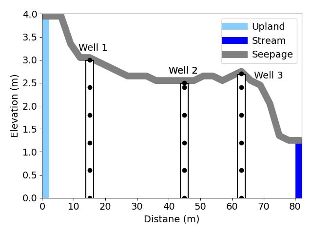
The system is a 2D cross-section from the upland to the stream with the same dimensions and elevation as the cross-section described in Yabusaki et al. (2020). The flow model has dimensions of 84 m 4 m and is defined on a grid with 28 40 cells. As shown in Fig. 1, the flow system is driven by Dirichlet pressure boundary conditions on the upland and stream sides. In contrast, a seepage boundary condition is applied to the ground surface and a no-flow boundary condition at the bottom. The source of salinity is the tidal stream, with the boundary conditions set based on one-year observations from hillslope wells and stream data Yabusaki et al. (2020). For more details on the model, please refer to Yabusaki et al. (2020).
Compared to the homogeneous case in Yabusaki et al. (2020), we simulate a more complicated heterogeneous field in this work. Figure 2 present three random realizations of log-permeability. These Gaussian realizations are generated using sequential Gaussian simulation with SGeMS Remy et al. (2009). The correlation lengths and are 5 and 5 grids, respectively. The mean and standard deviation of log-permeability (md) are 4.5 and 1, while the mean and standard deviation of porosity are 0.5 and 0.05. The same Gaussian field is used for both permeability and porosity, which serves as the input for the surrogate model. The other parameters are set based on Yabusaki et al. (2020). The model in Fig. 2(a) is used as the “true” model for data assimilation in Section 3.
The model is initially simulated for four years using annual observations to spin up the system to a dynamic steady state of groundwater levels, saturation, and total mass. After the spin-up, the simulation represents the initial freshwater conditions before seawater intrusion, which is then modeled over 7260 days (20 years). Monitoring wells, as shown in Fig. 1, are placed in the same locations as in Yabusaki et al. (2020) for model calibration and validation.


2.2 Surrogate Model Development using U-FNO
To efficiently address the uncertainty quantification and decision-making challenges in subsurface flow systems, it is necessary to discretize and solve equations 1 to 3 thousands to millions of times, which can be computationally prohibitive. To overcome this challenge, we develop a deep-learning-based surrogate model, U-FNO, to approximate the flow and transport processes for various permeability and porosity fields under consistent boundary conditions. The flow simulation process is expressed as
| (4) |
where denotes the geological model parameters (the permeability values in each cell, with as the total number of cells, and and denoting the number of cells in the 2D x-z domain), is the flow and transport simulation process, and represents the dynamic states of pressure and salinity in each cell over time steps.
The forward process can be approximated by a surrogate model as
| (5) |
where represents the approximate flow responses, denotes the surrogate model, and represents the parameters of the neural networks.
In this work, we apply the U-FNO framework proposed by Wen et al. (2022). The U-FNO architecture is modified based on the FNO Li et al. (2020) with modifications that append a U-Net to the Fourier layer to improve prediction accuracy. U-FNO is designed to conduct an infinite-dimensional-space input output mapping. The architecture of U-FNO used in this work is presented in Fig. 3. The geomodel input is discretized on the 2D domain and is repeated times as the function input for the networks. The input is then lifted to a higher-dimensional output through fully connected neural networks . Multiple iterative Fourier layers and U-Fourier layers are then applied to capture the spatio-temporal features of flow states. Another fully connected layer is applied in the end to map the U-Fourier layer output to surrogate model output .
In each Fourier layer , , the Fast Fourier Transform (FFT) is applied to the previous layer output to generate Fourier domain and capture the latent features. A linear transformation is then applied, followed by the inverse Fourier transform to map the Fourier domain back to the spatio-temporal domain. Additionally, a linear transform is applied directly to the function space and added to the output. The overall transformation process is written as
| (6) |
where denotes the activation function, is the number of Fourier layer used in U-FNO. K U-Fourier layers are applied after Fourier layers. U-Net is attached in each Fourier layer to improve the surrogate model performance. The output of U-Fourier layer is expressed as
| (7) |
for . The U-FNO architecture is written as
| (8) |
Please refer to Wen et al. (2022) for more details on U-FNO.

The training objective is to minimize the difference between the flow simulation output with the surrogate predictions from U-FNO. The minimization process of U-FNO parameters is described as
| (9) |
where is the number of training samples, is the extra weight applied to the data in the active cells . These active cells are determined based on the digital elevation model for the 2D vertical cross-section. The adaptive moment estimation (ADAM) in Kingma & Ba (2014) is applied to conduct the minimization process.
2.3 GeoFUSE: Data Assimilation Framework Utilizing ESMDA with Parameterization
To improve flow prediction accuracy, we apply data assimilation to calibrate the geological model, employing the GeoFUSE framework (Geological Forecasting using Surrogates and ESMDA). GeoFUSE integrates PCA for dimensionality reduction, the U-FNO surrogate model for high-fidelity flow prediction, and the ESMDA for iterative parameter calibration. This combination enables efficient model calibration, enhancing prediction accuracy while reducing uncertainty. A Bayesian framework is employed within the data assimilation process to generate posterior probability distributions.
In practical applications, monitoring data is collected from wells or geophysical observations. For synthetic cases like ours, the observed data is generated by adding random noise to a synthetic “true” model (Fig. 2(a)) as follows
| (10) |
where is the measurement error. When no structural bias is considered, the measurement error is assumed to be sampled from Gaussian distribution , where denotes the error covariance matrix. The posterior probability density function of model parameter conditioned to the observation using Bayesian framework is given by
| (11) |
where is the prior distribution of model parameters, is the likelihood function, and is a normalization factor that can be ignored.
Within the GeoFUSE framework as shown in Fig. 4, ESMDA Emerick & Reynolds (2013) is employed to sample posterior models, as illustrated in Eq. 11. Parameterization is generally needed to reduce the dimension of high-dimensional geological models and preserve the geological features. In this work, we consider a 2D Gaussian geomodel, and PCA is applied. The 2D geomodel can be generated from , where denotes the latent variables, denotes the basis matrix generated from singular value decomposition, and is the average value of model parameters. Using U-FNO as a surrogate model, the flow responses can be generated from .

In the GeoFUSE data assimilation framework, the latent variables are updated using
| (12) |
for and , where is the number of data assimilation steps, and is the number of ensemble realizations. In this work, we use , and the inflation coefficients are set to 4. And is the cross-covariance of latent variables and data variables , and is the data covariance matrix. These covariance matrices are updated at each assimilation step, corresponding to the updated ensemble. Random noise , sampled from a Gaussian distribution , is added in each iteration for mismatch calculation. After all assimilation steps are completed, the posterior models are generated using PCA on the posterior latent variables , and the posterior predictions are generated using U-FNO on the posterior models.
Figure 4 presents the GeoFUSE framework for data assimilation in the seawater intrusion problem. First, latent variables are sampled from a Gaussian distribution to generate a prior ensemble with samples. PCA is then applied to the latent variables to generate prior geomodels . The surrogate model is then applied to generate flow responses . ESMDA is performed, conditioned on the observations , to calibrate the latent variables . In each iteration, PCA and U-FNO are applied to generate pressure and salinity data that match the observations. After iterations, we generate posterior models and posterior predictions .
3 Results
The following section presents the prediction results, focusing on the performance of the U-FNO surrogate model, comparisons with PFLOTRAN simulations, and the model calibration and uncertainty reduction achieved through the GeoFUSE framework. These results highlight improvements in computational efficiency and predictive accuracy.
3.1 Surrogate Model (U-FNO) Training and Computational Efficiency
We simulate 1600 prior realizations to collect pressure and salinity data at 243 time steps, with measurements taken every 30 days. Of these, 1500 realizations are used to train the U-FNO-based surrogate model, while the remaining 100 are reserved for evaluating its predictive performance. The U-FNO architecture, comprising over 126 million parameters, is employed to train separate models for pressure and salinity outputs (Table 1).
The training process, conducted on a single Nvidia Tesla A100 GPU, takes 6.5 hours over 200 epochs for each network. In comparison, a full PFLOTRAN forward simulation required approximately 1.5 hours with one CPU. However, the U-FNO surrogate model predictions are computed in just 0.015 seconds, resulting in a computational speedup of around 360,000 times.
| Network | Layer | Output |
|---|---|---|
| Input | (40, 28, 243, 1) | |
| Padding | Padding | (40, 32, 248, 36) |
| Lifting | Linear | (40, 32, 248, 36) |
| Fourier layer 1 | Fourier3d/Conv1d/Add/ReLu | (40, 32, 248, 36) |
| Fourier layer 2 | Fourier3d/Conv1d/Add/ReLu | (40, 32, 248, 36) |
| Fourier layer 3 | Fourier3d/Conv1d/Add/ReLu | (40, 32, 248, 36) |
| U-Fourier layer 1 | Fourier3d/Conv1d/UNet3d/Add/ReLu | (40, 32, 248, 36) |
| U-Fourier layer 2 | Fourier3d/Conv1d/UNet3d/Add/ReLu | (40, 32, 248, 36) |
| U-Fourier layer 3 | Fourier3d/Conv1d/UNet3d/Add/ReLu | (40, 32, 248, 36) |
| Projection 1 | Linear | (40, 32, 248, 128) |
| Projection 2 | Linear | (40, 32, 248, 1) |
| Depadding | (40, 28, 243, 1) |
3.2 Comparisons of U-FNO Predictions and PFLOTRAN Simulations
To assess the predictive accuracy of the U-FNO surrogate model, we compare its results with the PFLOTRAN simulations. Figures 5 and 6 demonstrate the close agreement between the predicted and simulated salinity distributions over time and across multiple realizations in Fig. 2. The top row presents PFLOTRAN results, the middle row shows U-FNO predictions, and the bottom row highlights the absolute errors between the two. The comparisons are made for three key time points: 1050 days, representing the early-stage (approximately 3 years), 3570 days, marking the mid-stage (approximately 10 years), and 7170 days, indicating the late-stage (approximately 20 years), clearly illustrating the salinity dynamics over the 20-year period. As shown in Fig. 5, the U-FNO model effectively captures both the temporal and spatial dynamics of salinity. The absolute error for this realization falls in the middle range of the 100 test samples, demonstrating the model’s robustness in approximating complex flow and transport processes.


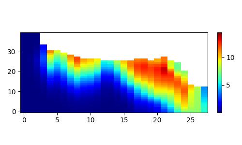


Figure 6 presents the variability in salinity plume size and shape across three different permeability realizations. This variability highlights the challenges of modeling heterogeneous systems, yet U-FNO successfully replicates these dynamics. The surrogate model consistently delivers high accuracy in its predictions, with the errors between U-FNO and PFLOTRAN being notably small, as shown in the bottom rows showing errors.


In addition to salinity distribution, Fig. 7 compares salinity accumulation between the U-FNO surrogate predictions and PFLOTRAN simulations for 100 test realizations. The results show the 10th, 50th, and 90th percentiles (P10, P50, and P90) over a period of 7,260 days. The black curves represent the PFLOTRAN results, while the blue dashed curves represent the U-FNO predictions. Over the 20-year period, the consistent increase in salinity accumulation and the close agreement between the surrogate model and full-scale simulations demonstrate the accuracy of U-FNO in approximating these long-term cumulative effects.

4 Uncertainty Reduction Through GeoFuse: Data Assimilation and Model Calibration
In the data assimilation process, pressure and salinity data are collected from three monitors at the locations shown as the black dots (18 monitoring locations in total) in Fig. 1. Data are collected monthly for the first five years, resulting in 2160 observations. To simulate realistic environmental conditions, Gaussian noise is added to the flow simulation results. We add Gaussian noise to the flow simulation results for the “true” model in Fig. 2(a). The standard deviation for the water level is set to 0.005 m, and for salinity, it is set to 0.2.
GeoFUSE effectively handles the high-dimensional geomodel parameters (permeability in each grid block) by reducing their dimension and enabling efficient parameter updates, with the latent dimension after PCA set to 642 based on energy criteria. The GeoFUSE framework applies ESMDA to assimilate observations over steps and calibrate the geological models. The data assimilation process results in more accurate predictions throughout the 20-year simulation period, conditioned on measurements from monitoring wells. The GeoFUSE framework significantly reduces the computational costs while delivering improved model and prediction accuracy for managing complicated subsurface environments.
Figure 8 shows the prior and posterior means and standard deviations of log-permeability. The prior models follow a Gaussian distribution, with the prior means close to the mean value of 4.5 and standard deviations near 1. The posterior means of the log-permeability parameters calibrated by GeoFUSE are closely aligned with the true geological model. The posterior models demonstrate substantial uncertainty reduction compared to the prior models, particularly in regions near the stream with high permeability. Additionally, the standard deviations of the posterior models are significantly reduced in areas of high permeability, indicating a marked decrease in uncertainty. These improvements highlight the effectiveness of the GeoFUSE framework in calibrating the geological model.


Results for salinity at the land surface of well 2 and salinity accumulation are shown in Fig. 9. Salinity accumulation refers to the total salinity in the entire region. The gray shaded area shows the P10 - P90 range of the prior. The black curves show the P10, P50, and P90 posterior results. The red dots show the observations, including random error, and the red curves show the true flow responses. Significant uncertainty reduction is achieved for both salinity at the well and salinity accumulation. Notably, even when the true salinity values fall outside the prior range, the posterior results still show substantial uncertainty reduction. These findings demonstrate the effectiveness of GeoFUSE in improving the accuracy and reliability of salinity predictions over the 20-year simulation period.


The clustering analysis using the K-means and K-medoids methods allows for generating representative salinity fields from both prior and posterior models. The K-means method is first applied to generate five clusters, and K-medoids is then used to select the center for each cluster. Figure 10 depicts the salinity fields from five representative clusters, showing how the posterior models more accurately capture the size and shape of the salinity plumes compared to the prior models. After applying GeoFUSE, the posterior models closely resemble the true salinity distributions, particularly in capturing larger and more distinct salinity plumes. This further demonstrates GeoFUSE’s capability to reduce uncertainty in the spatial distributions of state variables and effectively improve predictive accuracy.


These results collectively highlight the success of the GeoFUSE framework in significantly reducing computational costs, calibrating and reducing the uncertainty of geological models, and providing more reliable predictions of salinity distribution over the 20-year simulation period.
5 Discussion
5.1 Surrogate Model Accuracy and Limitations
The development of the U-FNO model represents a significant advancement in computational efficiency and accuracy for subsurface flow simulations. It achieves a remarkable speedup of approximately 360,000 times over traditional simulation models like PFLOTRAN, offering substantial benefits for large-scale simulations where computational resources and time are limited Wen et al. (2022). This efficiency is especially critical for scenarios requiring extensive Monte Carlo sampling for uncertainty quantification. As noted by Zhong et al. (2019), their cDC-GAN model similarly reduced simulation time, enabling numerous simulations for uncertainty analysis. However, U-FNO faces challenges in accurately predicting saltwater front movements, where its accuracy diminishes. This issue is not unique to U-FNO, as convolutional neural networks (CNN)-based methods Mo et al. (2019); Tang et al. (2020) have exhibited similar discrepancies when approximating multiphase flow behaviors in heterogeneous systems. Despite these challenges, U-FNO’s overall predictive accuracy remains impressive, making it a transformative tool for large-scale, data-intensive studies.
5.2 Effectiveness of GeoFUSE
The GeoFUSE framework substantially accelerates the subsurface flow modeling and data assimilation process while significantly reducing the uncertainty in geological models and long-term predictions, particularly for seawater intrusion and groundwater management in coastal areas. This approach aligns with previous studies that emphasize the importance of addressing geological uncertainty to enhance predictive capabilities Sonnenborg et al. (2015); He et al. (2015). Within the GeoFUSE framework, PCA is used to reduce the dimension of geological models while preserving essential features, enabling more efficient uncertainty quantification for large-scale Gaussian models. Additionally, the ability of ESMDA to assimilate sparse and noisy data makes the framework both simple and robust for subsurface flow predictions. The results, which show improved salinity distribution predictions over a 20-year simulation period, further highlight the framework’s effectiveness in model calibration and uncertainty reduction. Overall, GeoFUSE provides a transformative approach to subsurface flow simulations and uncertainty quantification in complex coastal environments by accelerating flow and transport simulations, efficiently calibrating geological models, and reducing the uncertainty of future predictions.
5.3 Implications for Seawater Intrusion and Floodplain Management
GeoFUSE offers a powerful tool for decision-makers involved in floodplain management, tidal restoration, and salinity control by providing rapid and accurate predictions and model calibrations. This capability enhances water resource management in the face of rising sea levels and climate change. By offering predictive modeling for salinity intrusion in vulnerable coastal regions, GeoFUSE plays a critical role in broader coastal management efforts. Its ability to deliver timely, accurate insights makes it essential for adaptive management, especially as seawater intrusion intensifies due to climate change. This allows decision-makers to respond swiftly to evolving conditions in coastal aquifers.
The integration of monitoring data into predictive models, as demonstrated in this study, significantly reduces model uncertainty and improves the management of coastal aquifers. GeoFUSE’s use of a surrogate model reduces computational costs, enabling rapid predictions for uncertainty quantification and decision-making. By assimilating monitoring data, the framework improves salinity forecasts by reducing uncertainty in the geological models. The model’s performance, validated against PFLOTRAN simulation results and prior statistics, confirms its predictive accuracy and robustness in model calibration.
5.4 Future Work, Model Scalability, and Caveats
GeoFUSE has demonstrated substantial potential in subsurface flow modeling and uncertainty quantification, but there is room for further improvement and scalability. One area of focus is refining the U-FNO model, which has effectively captured complex multiphase flow dynamics Wen et al. (2022). However, further adjustments could enhance its ability to account for fine-scale geological variations, which are crucial in heterogeneous environments. Additionally, incorporating more complex factors, such as boundary conditions influenced by climate change, could increase the model’s robustness. Climate-induced variability significantly impacts hydrological cycles and groundwater dynamics He et al. (2015), and addressing these complexities would enable GeoFUSE to more accurately simulate the intricate interactions between geological formations and hydrological processes across diverse environments.
Future research could also focus on extending GeoFUSE to three-dimensional (3D) models, which are essential for accurately simulating subsurface flow in coastal regions increasingly affected by seawater intrusion. Recent studies highlight the importance of 3D geological modeling in understanding fluid dynamics and permeability in geothermal systems Siler et al. (2019); Torresan et al. (2020). A 3D framework would better integrate geological, geophysical, and geochemical data, providing a more comprehensive approach to evaluating both anthropogenic and natural influences on subsurface flow Strati et al. (2017); Dwivedi et al. (2018). By improving scalability and addressing these key areas, GeoFUSE could evolve in a versatile tool for groundwater management in diverse environments, particularly in coastal regions facing challenges such as groundwater depletion and climate change Messier et al. (2015); Ebong et al. (2020).
6 Concluding Remarks
In this work, we developed a novel framework, GeoFUSE, to address the computational challenges associated with seawater intrusion modeling in coastal aquifers. GeoFUSE integrates the U-FNO surrogate model for fast spatio-temporal predictions with ESMDA for data assimilation and model calibration. The framework was applied to a 2D cross-section of a tidal stream-floodplain system, predicting pressure and salinity responses while accounting for geological heterogeneity and uncertainty in flow responses. The GeoFUSE approach enabled efficient data assimilation, with PCA parameterizing Gaussian geological models and ESMDA calibrating heterogeneous models for posterior sampling.
We trained the U-FNO model using 1500 realizations and demonstrated its ability to significantly reduce computational costs compared to PFLOTRAN simulations while maintaining predictive accuracy. The data assimilation framework was used to calibrate the geological models based on five years of observation data from three wells and predict salinity distribution and accumulation over a 20-year period. Results showed substantial uncertainty reduction for both models and flow responses, highlighting the effectiveness and efficiency of GeoFUSE.
Future work will focus on extending GeoFUSE to large 3D models and incorporating more complex boundary conditions, including the impacts of climate change, sea-level rise, and extreme weather events. Expanding the framework to include pumping and injection strategies for seawater intrusion mitigation, as well as uncertainty quantification for optimization, will further enhance real-time predictions and decision-making processes. While training deep learning models like U-FNO can introduce uncertainty due to the variability in training data from geological models, GeoFUSE holds great promise for advancing large-scale subsurface flow and transport simulations with improved accuracy.
Data Availability Statement
The simulation data can be generated by solving the equations using the input parameters presented in the figures and methodology. Data will be made available upon request. The code used in this study will be shared in a GitHub repository by the time of publication.
Acknowledgements.
This work was supported by the Automated Scenario Assessment of Groundwater Table & Salinity Response to Sea-Level Rise Project at Lawrence Berkeley National Laboratory, funded by the U.S. Department of Defense, Strategic Environmental Research and Development Program (SERDP).References
- Arora et al. ((2012)) Arora, B., Mohanty, B. & McGuire, J. (2012). Uncertainty in dual permeability model parameters for structured soils. Water Resources Research 48 1 .
- Arora et al. ((2011)) Arora, B., Mohanty, B.P. & McGuire, J.T. (2011). Inverse estimation of parameters for multidomain flow models in soil columns with different macropore densities. Water resources research 47 4 .
- Bhattacharjya & Datta ((2009)) Bhattacharjya, R.K. & Datta, B. (2009). ANN-GA-based model for multiple objective management of coastal aquifers. Journal of Water Resources Planning and Management 135 5 314–322.
- Cao et al. ((2024)) Cao, C., Zhang, J., Gan, W., Nan, T. & Lu, C. (2024). A deep learning-based data assimilation approach to characterizing coastal aquifers amid non-linearity and non-Gaussianity challenges. Water Resources Research 60 7 e2023WR036899.
- Dodangeh et al. ((2022)) Dodangeh, A., Rajabi, M.M., Carrera, J. & Fahs, M. (2022). Joint identification of contaminant source characteristics and hydraulic conductivity in a tide-influenced coastal aquifer. Journal of Contaminant Hydrology 247 103980.
- Dwivedi et al. ((2018)) Dwivedi, D., Arora, B., Steefel, C.I., Dafflon, B. & Versteeg, R. (2018). Hot spots and hot moments of nitrogen in a riparian corridor. Water Resources Research 54 1 205–222.
- Ebong et al. ((2020)) Ebong, E.D., Akpan, A.E. & Ekwok, S.E. (2020). Stochastic modelling of spatial variability of petrophysical properties in parts of the Niger Delta Basin, southern Nigeria. Journal of Petroleum Exploration and Production Technology 10 569–585.
- Emerick & Reynolds ((2013)) Emerick, A.A. & Reynolds, A.C. (2013). Ensemble smoother with multiple data assimilation. Computers & Geosciences 55 3–15.
- Goebel et al. ((2017)) Goebel, M., Pidlisecky, A. & Knight, R. (2017). Resistivity imaging reveals complex pattern of saltwater intrusion along Monterey coast. Journal of Hydrology 551 746–755.
- Hammond et al. ((2014)) Hammond, G.E., Lichtner, P.C. & Mills, R. (2014). Evaluating the performance of parallel subsurface simulators: An illustrative example with PFLOTRAN. Water Resources Research 50 1 208–228.
- Han et al. ((2024)) Han, Y., Hamon, F.P., Jiang, S. & Durlofsky, L.J. (2024). Surrogate model for geological CO2 storage and its use in hierarchical MCMC history matching. Advances in Water Resources 187 104678.
- He et al. ((2015)) He, X., Højberg, A.L., Jørgensen, F. & Refsgaard, J.C. (2015). Assessing hydrological model predictive uncertainty using stochastically generated geological models. Hydrological Processes 29 19 4293–4311.
- Hussain et al. ((2015)) Hussain, M.S., Javadi, A.A., Ahangar-Asr, A. & Farmani, R. (2015). A surrogate model for simulation–optimization of aquifer systems subjected to seawater intrusion. Journal of Hydrology 523 542–554.
- Jiang & Durlofsky ((2023)) Jiang, S. & Durlofsky, L.J. (2023). Use of multifidelity training data and transfer learning for efficient construction of subsurface flow surrogate models. Journal of Computational Physics 474 111800.
- Jiang & Durlofsky ((2024)) Jiang, S. & Durlofsky, L.J. (2024). History matching for geological carbon storage using data-space inversion with spatio-temporal data parameterization. International Journal of Greenhouse Gas Control 134 104124.
- Ketabchi et al. ((2016)) Ketabchi, H., Mahmoodzadeh, D., Ataie-Ashtiani, B. & Simmons, C.T. (2016). Sea-level rise impacts on seawater intrusion in coastal aquifers: Review and integration. Journal of Hydrology 535 235–255.
- Kingma & Ba ((2014)) Kingma, D.P. & Ba, J. (2014). Adam: A method for stochastic optimization. arXiv preprint arXiv:1412.6980 .
- Langevin & Guo ((2006)) Langevin, C.D. & Guo, W. (2006). MODFLOW/MT3DMS–based simulation of variable-density ground water flow and transport. Groundwater 44 3 339–351.
- Langevin et al. ((2008)) Langevin, C.D., Thorne Jr, D.T., Dausman, A.M., Sukop, M.C. & Guo, W. (2008). SEAWAT version 4: a computer program for simulation of multi-species solute and heat transport Tech. Rep.. : Geological Survey (US).
- Li et al. ((2020)) Li, Z., Kovachki, N., Azizzadenesheli, K., Liu, B., Bhattacharya, K., Stuart, A. & Anandkumar, A. (2020). Fourier neural operator for parametric partial differential equations. arXiv preprint arXiv:2010.08895 .
- Meray et al. ((2024)) Meray, A., Wang, L., Kurihana, T., Mastilovic, I., Praveen, S., Xu, Z.Wainwright, H. (2024). Physics-informed surrogate modeling for supporting climate resilience at groundwater contamination sites. Computers & Geosciences 183 105508.
- Messier et al. ((2015)) Messier, K.P., Campbell, T., Bradley, P.J. & Serre, M.L. (2015). Estimation of groundwater Radon in North Carolina using land use regression and Bayesian maximum entropy. Environmental Science & Technology 49 16 9817–9825.
- Mo et al. ((2019)) Mo, S., Zabaras, N., Shi, X. & Wu, J. (2019). Deep autoregressive neural networks for high-dimensional inverse problems in groundwater contaminant source identification. Water Resources Research 55 5 3856–3881.
- Provost & Voss ((2019)) Provost, A.M. & Voss, C.I. (2019). SUTRA, a model for saturated-unsaturated, variable-density groundwater flow with solute or energy transport—documentation of generalized boundary conditions, a modified implementation of specified pressures and concentrations or temperatures, and the lake capability Tech. Rep.. : US Geological Survey.
- Rajabi & Ketabchi ((2017)) Rajabi, M.M. & Ketabchi, H. (2017). Uncertainty-based simulation-optimization using Gaussian process emulation: application to coastal groundwater management. Journal of Hydrology 555 518–534.
- Remy et al. ((2009)) Remy, N., Boucher, A. & Wu, J. (2009). Applied geostatistics with SGeMS: A user’s guide. : Cambridge University Press.
- Siler et al. ((2019)) Siler, D.L., Faulds, J.E., Hinz, N.H., Dering, G.M., Edwards, J.H. & Mayhew, B. (2019). Three-dimensional geologic mapping to assess geothermal potential: Examples from Nevada and Oregon. Geothermal Energy 7 1–32.
- Sonnenborg et al. ((2015)) Sonnenborg, T., Seifert, D. & Refsgaard, J. (2015). Climate model uncertainty versus conceptual geological uncertainty in hydrological modeling. Hydrology and Earth System Sciences 19 9 3891–3901.
- Sreekanth & Datta ((2010)) Sreekanth, J. & Datta, B. (2010). Multi-objective management of saltwater intrusion in coastal aquifers using genetic programming and modular neural network based surrogate models. Journal of Hydrology 393 3-4 245–256.
- Strati et al. ((2017)) Strati, V., Wipperfurth, S.A., Baldoncini, M., McDonough, W.F. & Mantovani, F. (2017). Perceiving the crust in 3-D: A model integrating geological, geochemical, and geophysical data. Geochemistry, Geophysics, Geosystems 18 12 4326–4341.
- Tang et al. ((2020)) Tang, M., Liu, Y. & Durlofsky, L.J. (2020). A deep-learning-based surrogate model for data assimilation in dynamic subsurface flow problems. Journal of Computational Physics 413 109456.
- Torresan et al. ((2020)) Torresan, F., Piccinini, L., Pola, M., Zampieri, D. & Fabbri, P. (2020). 3D hydrogeological reconstruction of the fault-controlled Euganean Geothermal System (NE Italy). Engineering Geology 274 105740.
- Wen et al. ((2022)) Wen, G., Li, Z., Azizzadenesheli, K., Anandkumar, A. & Benson, S.M. (2022). U-FNO—an enhanced Fourier neural operator-based deep-learning model for multiphase flow. Advances in Water Resources 163 104180.
- Werner et al. ((2013)) Werner, A.D., Bakker, M., Post, V.E., Vandenbohede, A., Lu, C., Ataie-Ashtiani, B.Barry, D.A. (2013). Seawater intrusion processes, investigation and management: Recent advances and future challenges. Advances in Water Resources 51 3–26.
- Yabusaki et al. ((2020)) Yabusaki, S.B., Myers-Pigg, A.N., Ward, N.D., Waichler, S.R., Sengupta, A., Hou, Z.others (2020). Floodplain inundation and salinization from a recently restored first-order tidal stream. Water Resources Research 56 7 e2019WR026850.
- Yoon et al. ((2017)) Yoon, S., Williams, J.R., Juanes, R. & Kang, P.K. (2017). Maximizing the value of pressure data in saline aquifer characterization. Advances in Water Resources 109 14–28.
- Zhong et al. ((2019)) Zhong, Z., Sun, A.Y. & Jeong, H. (2019). Predicting CO2 plume migration in heterogeneous formations using conditional deep convolutional generative adversarial network. Water Resources Research 55 7 5830–5851.
- Zhou & Tartakovsky ((2021)) Zhou, Z. & Tartakovsky, D.M. (2021). Markov chain Monte Carlo with neural network surrogates: Application to contaminant source identification. Stochastic Environmental Research and Risk Assessment 35 639–651.
- Zhou et al. ((2022)) Zhou, Z., Zabaras, N. & Tartakovsky, D.M. (2022). Deep learning for simultaneous inference of hydraulic and transport properties. Water Resources Research 58 10 e2021WR031438.