

Abstract
The inverse problem of estimating the background potential from measurements of the local density of states is a challenging issue in quantum mechanics. Even more difficult is to do this estimation using approximate methods such as scanning gate microscopy (SGM). Here, we propose a machine-learning-based solution by exploiting adaptive cellular neural networks (CNNs). In the paradigmatic setting of a quantum point contact, the training data consist of potential-SGM functional relations represented by image pairs. These are generated by the recursive Green’s function method. We demonstrate that the CNN-based machine learning framework can predict the background potential corresponding to the experimental image data. This is confirmed by analyzing the estimated potential with image processing techniques based on the comparison between the charge densities and those obtained using different techniques. Correlation analysis of the images suggests the possibility of estimating different contributions to the background potential. In particular, our results indicate that both charge puddles and fixed impurities contribute to the spatial patterns found in the SGM data. Our work represents a timely contribution to the rapidly evolving field of exploiting machine learning to solve difficult problems in physics.

Original content from this work may be used under the terms of the Creative Commons Attribution 4.0 license. Any further distribution of this work must maintain attribution to the author(s) and the title of the work, journal citation and DOI.
1. Introduction
Recent years have witnessed a growing interest in exploiting machine learning techniques to solve difficult problems in physics. Examples include the application of deep learning to experimental particle physics [1, 2], solving quantum many-body problems with artificial neural networks [3], the inverse design of photonic and optical systems [4] and using machine learning and artificial intelligence in quantum information science and technology [5, 6]. In nonlinear dynamical systems, recurrent neural networks, such as echo state machines [7] (or reservoir computing machines) have been adopted to predict the state evolution of chaotic systems [8–14]—a problem deemed fundamentally challenging due to the hallmark of chaos: sensitive dependence on initial conditions. Physical principles have also been incorporated into machine learning, leading to physics-enhanced machine learning, as exemplified by Hamiltonian neural networks [15–19].
In this paper, we develop a machine-learning framework to solve a standing inverse problem in solid-state quantum devices inferring the background potential from experimental image data related to the local density of states (LDOS). When a quantum device, such as a quantum point contact (QPC) or a quantum dot has been fabricated, it is of great experimental and theoretical interest to determine the details of and the contributing factors to the intrinsic background potential that would affect the transport properties of the device. In this regard, the standard technique used to infer the LDOS is scanning gate microscopy (SGM), where a charged tip rasters a device to measure fluctuations in its conductance. Typically, a weak electrical potential is applied to the tip and it hovers a few nanometers above the surface of the device so that its coupling is weak and the potential can be regarded as a small perturbation to the Fermi sea. Under stringent conditions, the conductance fluctuations are approximately proportional to the LDOS [20–23]. The SGM makes it possible to infer certain properties of quantum constrictions, such as quantum interference patterns [24–26], compressibility zones in the quantum Hall regime [27] and large-scale features of the background potential [28, 29] (see [30] for a comprehensive review of the SGM technique).
Our question is as follows: given the SGM-generated images, can the detailed background potential be inferred? This is a challenging inverse problem in quantum mechanics, for which previous machine-learning solutions were devised but for 1D problems only, such as those based on multilayered neural networks [31] or the nonparametric Bayesian approximation [32]. Bayesian estimation, in particular, has been applied to other problems in solid state physics [33, 34], but this is a method that has some limitations depending on the level of complexity of the problem at hand. For instance, it is typically difficult to cover the whole hypothesis space or guess appropriate priors. In addition, for parametric estimation, the number of parameters may render the problem intractable.
Here, we propose to exploit a supervised learning approach based on an alternative architecture, cellular neural networks (CNNs) to infer the background potential of 2D quantum devices from SGM images. CNNs are cellular automata that are also nonlinear dynamical systems with deterministic rules on a discrete grid capable of reproducing the behavior of a large class of dynamical systems [35–38]. Due to its distributed architecture designed for massively parallel processing, CNNs have been used to solve problems such as image deconvolution [39], the Ising model [40] and fluid dynamics [41].
To adapt the CNNs to our quantum inverse problem, we first build up a theoretical database of potential-SGM image pairs by using the standard Green’s function approach [42, 43] and use them as our ground truth. We then train the CNN with the data set to make it learn how to translate the latter into the former. Once trained with theoretical data, the CNN model is transferred to make predictions of the background potential from experimental SGM data that it has never seen. CNN-generated potential images enable further analysis to determine the main physical factors that contribute to the background potential—an appealing feature of our machine-learning-based method.
2. Method
That the SGM-measured conductance fluctuations are proportional to the LDOS can be seen, intuitively, as follows. When treated as a small perturbation, the tip potential causes a small shift of the eigenenergies of the quantum device by,

where n is the mode being analyzed and V is the perturbation potential. For the rastering tip, this potential can be approximated as  . The energy shifts become:

where  is the wave function evaluated at the tip position r0. At low temperatures, transport across the device occurs at the surface of the Fermi sea, so the changes in the conductance can be approximated by:

Thus, it can be seen that the SGM-generated variations or fluctuations in conductance are approximately proportional to the LDOS. More detailed calculations confirmed this heuristic relation [20–23].
However, it is difficult to meet all the following requirements: (a) a sufficiently weak perturbation, (b) a delta-shaped induced potential, (c) a wave function given by states at the Fermi energy. On the other hand, a strong correspondence between the SGM image and the LDOS can be obtained when the depletion disk created by the tip has a radius smaller than the Fermi wavelength [21]. Nonetheless, wave function scarring and localized states are typically robust and produce good agreement between the LDOS and SGM images [22].
To alleviate these restrictions, we still treat the tip potential as a perturbation, but we generate theoretical SGM images instead of calculating the LDOS. Next, we discuss the prototypical device used in this study and then detail the theoretical approach.
2.1. QPC as a prototypical device
We use a QPC as a prototype device to demonstrate the operation of our machine-learning approach to finding the background potential. The QPC is fabricated in an In0.53Al0.47As/In0.53Ga0.47As/In0.53Al0.47As modulation-doped heterostructure, as previously reported [25]. The calculated electron density is  cm−2, which gives a mean-free path of 1.2 µm and a Fermi wavelength of
  nm, which is approximately the diameter of the scanning tip.
The scanned area is  µm2 and the QPC is formed with in-plane gates defined by 100 nm deep trenches, as shown in the atomic force microscopy (AFM) topographic image in the inset of figure 1. The device is coated with approximately 30 nm of polymethylmethacrylate (PMMA) for protection. The SGM is performed hovering a PtIr-coated tip 40 nm above the surface. All images were taken at 280 mK.

Figure 1. Transmission curve of the prototypical device, a QPC with disorder used to demonstrate our machine-learning approach to find the background potential. Red disks indicate at what transmissions and side gate voltages the SGM images were taken. Gray shading indicates the regions where the neural network was trained. Inset shows a  µm2 AFM topographic image of the device. Shaded region corresponds to an area of
  nm2 where the computations are performed. Blue regions are etched trenches that define the side gates.
Download figure:
Standard image High-resolution imageBased on the experimental images, we produced a  grid for a region of
  nm2 indicated in figure 1. This gives a discretization step of 1.125 nm corresponding to a wavenumber of 0.21 nm−1, which is far from the edge of the first Brillouin zone at 5.58 nm−1. In all simulations, we applied a saddle potential to the whole region described by,

where  meV,
meV,  point to the center of the region, and
  are the potential strengths so that
  meV and
  meV.
meV.
2.2. Generating training data using the Green’s function method
Beyond the saddle potential, an additional random potential is added to simulate the presence of charged impurities in the sample. It is created using a ‘percolation’ approach where each site of the simulation grid is filled with a single impurity with a constant probability ![$p\in[0,0.04]\%$](https://content.cld.iop.org/journals/2632-2153/3/2/025013/revision2/mlstac6ec7ieqn13.gif) . In this way, it is possible to produce additional potentials ranging from isolated impurities to clusters of impurities. When a site is selected, a Coulomb-like potential (
. In this way, it is possible to produce additional potentials ranging from isolated impurities to clusters of impurities. When a site is selected, a Coulomb-like potential ( ) is created around it with a radius of five lattice constants and a maximum truncated value of 10 meV at the site. The variations in the random potential are likely to have a resolution of the order of the Bohr radius (
 ). This, for the InGaAs heterostructure, is approximately 18 nm given a specific mass of 0.041 [44], which corresponds to a radius of approximately eight lattice constants, which can be fully captured by our Coulomb-like potential.
The training data consist of a large number of ‘image functions’ (calculated SGM patterns) of the different potentials, which are calculated using the standard recursive Green’s function approach [42, 43, 45]. In particular, we divide the effective device region into several transverse segments and calculate the Green’s function from the left and right leads. The new segments are progressively attached to both leads until they meet together in a single segment at which the image is calculated. Mathematically, the corresponding Dyson’s equation is,

where  is the coupling matrix between segments a and b, and the zero superscript indicates the unperturbed Green’s function given by:

with  and Hn
being the Hamiltonian for the nth segment.
and Hn
being the Hamiltonian for the nth segment.
We model the tip potential with,

where d0 is a fixed parameter set to 80 lattice constants,  and
and  give the location of the scanning tip, and x and y give an arbitrary position around a disk centered on
  with a radius of 14 lattice constants (
 real tip radius).
In the weak perturbation approximation given by equation (3), the change in conductance is proportional to the sum of the LDOS weighted by the corresponding tip potential at each site. It is important to point out that this is a weak approximation, but more precise calculations make the procedure unfeasible with current technology due to the long simulation times. However, using the Green’s function approach, the LDOS is given by,

The transmission at a specific energy is given by:

where ![$\Gamma_{\text{L,R}} = i\left[\Sigma_{\text{L,R}}-\Sigma_{\text{L,R}}^{\dagger}\right]$](https://content.cld.iop.org/journals/2632-2153/3/2/025013/revision2/mlstac6ec7ieqn22.gif) ,
,  is the self-energy of each lead, and GLR is the Green function connecting the left and right leads.
This procedure requires the ‘initial’ state, i.e. the lead Green’s functions denoted as  , which can be calculated semi-analytically using the method of mode representation [43]. In all computations, the Fermi energy is randomly chosen so that the maximum transmission is eight, which is an experimental limitation.
We separated theoretical potential-LDOS image pairs into eight groups ![$(t,t+1],\ \forall t = 0,1,\dots, 8$](https://content.cld.iop.org/journals/2632-2153/3/2/025013/revision2/mlstac6ec7ieqn27.gif) , according to their corresponding transmission t. For each group, at least 200 pairs were generated and increased to 1600 by applying a combination of horizontal/vertical flipping and salt-and-pepper noise. Therefore, 12 800 image pairs were created in total.
, according to their corresponding transmission t. For each group, at least 200 pairs were generated and increased to 1600 by applying a combination of horizontal/vertical flipping and salt-and-pepper noise. Therefore, 12 800 image pairs were created in total.
2.3. Cellular neural networks
The state X of a cell in this architecture evolves according to,


where  is the Moore neighborhood around the cell (i, j), Z is an offset set to one, the tensors A and B are known as the ‘cloning template’,
  is the input of the automata and
  is its output. We use the CNN as an image translator, feeding the SGM image to the input U of the network and obtaining the potential from its output Y. However, note that although our problem is time independent, the CNN algorithm is a dynamical system. Nonetheless, for fixed inputs, as in this case, the output converges to a fixed value, and it is exactly the steady-state value of Y that we use as output (potential).
A pictorial representation of this architecture is illustrated in figure 2. In the standard CNN algorithm, a bipolar clamped activation is used as the output. In our study, we use,


Figure 2. Schematic illustration of the CNN. Dynamical state of the central cell is Xij and its eight directly connected cells constitute its Moore neighborhood.
Download figure:
Standard image High-resolution image2.3.1. Inferring step
In an inferring step, where we want to infer the potential given an SGM image, we discretize the equations using finite differences and use the Euler method to find,

where

 or
or  indicates the contraction between a tensor and a multidimensional array, and J is the full rank matrix of ones. The step size Δ is an adimensional hyperparameter of the network that defines its update rate. In the Euler method, the step size sets the upper-bound error of the numerical procedure. Therefore, choosing small values of Δ results in a better approximation at the cost of longer procedures. We use a constant
  in all operations of the CNN.
In a typical procedure, we evolve the state of the whole grid using Dirichlet boundary conditions until  is achieved. In all simulations, we used
  as a stopping criterion. The step at which this condition is satisfied we denote by N.
2.3.2. Correcting step
Training the network has the objective of finding a cloning template that makes the CNN better predict the potential given an SGM image. This is accomplished by feeding the network with an SGM image, inferring the potential, and calculating the correlation rXP between the state X and the expected potential P:
We then use a standard gradient descent strategy to update the cloning template:


where η is the ‘training rate’ of the network, which is fixed at  . Specifically, we use the following gradients:


where σ is the standard deviation of all elements of the multidimensional array.
However, we only update the gradients after 14 inferring/correcting steps with different randomly chosen training potential-SGM image pairs.
The training of the network is regarded as being complete when the correlation between the images reaches a steady value  %. After each epoch (steps = number of image pairs divided by 14), a set of 100 SGM images never before seen by the CNN are fed to the network, and an average test error is calculated.
3. Results
After training the network with pairs from a specific transmission block, we feed it with experimental SGM images obtained at a base transmission within that block (see figure 1) and estimate the corresponding potential.
To achieve this, we normalized the experimental data to fit the numerical range between −1 and +1. In addition, the pixelwise average and the variance of the predicted potentials over all experimental SGM data are computed. These last two images are shown in figures 3(a) and (b), respectively. The average of the predicted potentials (from the CNN) in figure 3(a) shows a horizontal region where most of the patterns are visible. The top and bottom ~50 nm regions are dominated by the saddle potential (equation (4)) that depletes the LDOS. Consequently, not much variability in the LDOS training set exists in these regions and the inference for the potential in these limits is not reliable. Hence, all analyses must be performed between 50–625 nm vertically. The variance in the predicted potentials in figure 3(b) confirms this observation and indicates high variability of possible defects.

Figure 3. Typical set of results: (a) pixelwise average and (b) variance of all predicted potential images over all different experimental SGM  images as inputs of the CNN, (c) experimental SGM
  image obtained with a side-gate voltage of −4 V, corresponding to a conductance of
  without the scanning tip. Image was obtained with a tip voltage of −0.5 V, as previously reported [30] and (d) the corresponding potential image predicted by the CNN.
Download figure:
Standard image High-resolution imageFigures 3(c) and (d) show a typical experimental  SGM image (measured changes in conductance as the tip scans the device) and the corresponding potential predicted by the CNN, respectively. The SGM image was obtained with a side-gate voltage of −4 V, which corresponds to a base conductance of
  (
( ) without the scanning tip. The image was obtained with a tip voltage of −0.5 V, as previously reported [30].
Our CNN-based method can be used to estimate the density of fixed charges coming from either impurities or charge puddles in the 2D electron gas. Whereas the former presents itself as recalcitrant features in all potential images, the latter changes depending on the input SGM image.
Previous attempts to quantify the density of impurities were based on examining conductance fluctuations [46]. However, we base our estimate on the Shannon entropy [47] of the potential image defined as the expected value of the information content  of an image Y:

where pi
is the frequency of the intensity level i of the image, and the information content for a bin i is given by the self-information  . The latter measures the uncertainty of information at a specific bin. For instance, if
  , the self-information is zero, while if there are two equally possible outcomes, then
  and the self-information is 1. When the latter happens, the product
  gives
gives  and S sums up to 1. Since we are using base 2, this gives the number of bits necessary to store this information. When applied to the whole image, the Shannon entropy gives the total number of bits necessary to represent the image.
Since an image can be represented by S bits and we have a maximum of 8 bits per pixel, the number of impurities in the image is  (number of data points in an experimental SGM reading) and the density is estimated by,

Figure 4 shows the estimated density for different gate voltages. The fixed charge density is in the order of 1011 cm−2, which is a fraction of the doping density for this heterostructure (7.2 × 1011 cm−2). Moreover, the fixed charge concentration decreases as the QPC is squeezed as a consequence of depletion.

Figure 4. Estimated fixed charge density as a function of the side-gate voltage. Dashed line is a linear fitting of the experimental data, indicating a decreasing trend as the QPC is squeezed.
Download figure:
Standard image High-resolution image3.1. Clustering analysis
To identify the physical factors that contribute to the background potential, we calculate the cluster distribution of the estimated potentials. Here, a cluster is defined as a group of nearest neighboring sites whose potentials differ at the most by  . We use an intensity-based spatial clustering algorithm where features with similar intensities are grouped if the size of the proposed cluster is larger than a predetermined threshold (
 pixels), otherwise the pixels are considered noise and are not grouped. This algorithm is based on the standard DBSCAN [48]. Therefore, the average cluster mass (number of pixels in a cluster) is calculated as,

where p(i) is the probability of finding a cluster of mass i.
A complementary study is performed by checking the structure of such clusters. A measure of how much the clusters cover the potential image depending on the scale is known as the Minkowski–Bouligand dimension (or box dimension). We estimate the box dimension using a box-counting algorithm, where we count the number N of boxes of side  that are necessary to cover all filled sites. This is widely used in percolation theory, for instance, to identify percolating clusters. The box dimension is then given by,

The average cluster mass and the Minkowski–Bouligand dimension for the largest cluster are shown in figure 5. As the QPC is squeezed by side-gate potentials, the average cluster mass increases, and this is mirrored by an increase in the Minkowski–Bouligand dimension. Figure 5 also shows that a small gate voltage ( V) is enough to rapidly change the complexity of the background potential, leading to the appearance of broad features. This suggests that potential images obtained for high gate voltages may be dominated by static impurity charges.

Figure 5. Analysis of potential images. Shown are the average cluster mass and the Minkowski–Bouligand dimension for the CNN estimated potential images. Insets show the channel at several specific gate voltage values as indicated by the dashed line. In both cases, dots are experimental data, whereas the dotted curves are spline interpolations.
Download figure:
Standard image High-resolution image3.2. Correlation analysis
To check for similar structures in different images, we organize the predicted potential images (matrices) in ascending order according to the side-gate voltage and define an image–image correlation function as,

where the outer average is performed over all matrix elements, σ is the standard deviation and  is the vectorization of matrix Yi
. Since every image Yi
is predicted for a specific side-gate voltage, we can map the index k to an offset voltage. The image–image autocorrelation function as a function of the offset voltage is shown in figure 6.
is the vectorization of matrix Yi
. Since every image Yi
is predicted for a specific side-gate voltage, we can map the index k to an offset voltage. The image–image autocorrelation function as a function of the offset voltage is shown in figure 6.
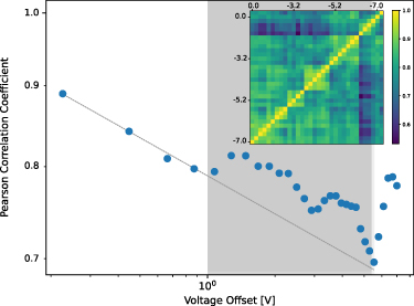
Figure 6. Image–image correlation function versus the offset voltage. Shaded area corresponds to a region where the correlation diverges from a power-function trend. Inset shows the similarity matrix for the potential images.
Download figure:
Standard image High-resolution imageA complementary measure is given by the self-similarity matrix that quantifies the similarity between images. It is defined as,

The image–image correlation and the similarity matrix for our data are shown in figure 6. The autocorrelation function decays approximately as a power function with a tail coefficient of −0.0125. However, there are three distinct regions. For voltage offsets below approximately 1 V, the correlation function decays at a nearly constant rate, which is related to a change in the background potential possibly related to charge puddles. Offset voltages between approximately 1–5.5 V show an increase in correlation, which may be related to the appearance of novel features. Offset voltages higher than 5.5 V display a sudden increase in correlation indicating the appearance of invariant features in the estimated potential. This behavior is also captured by the similarity matrix shown in the inset of figure 6.
3.3. Pinch-off region
To complete the analysis, we study the estimated potential image near the pinch-off region of the QPC. To obtain the recalcitrant features revealed by the image–image correlation function for high gate voltages, we discarded the noise in the images and studied only clusters with mass larger than  pixels.
Figure 7(a) shows the SGM image obtained from a gate voltage of −7.4 V, while figure 7(b) shows potential islands corresponding to the fixed impurity regions. The CNN approach suggests that the broad and bold features obtained by SGM indicate a high-potential region that blocks the electron flow, as previously speculated [28]. It is also important to note that this spatial cluster configuration is mostly unaffected by side-gate voltages higher than −6.5 V.

Figure 7. Analysis of the estimated potential image near the QPC pinch-off region. (a) Experimental SGM image of the QPC near pinch-off where the applied gate voltage is −7.4 V. (b) Corresponding estimated potential image (from the CNN) where only clusters with a mass larger than  pixels are colored.
Download figure:
Standard image High-resolution image
4. Conclusion
We have articulated a machine-learning method to address the inverse problem of determining the background potential from experimentally measured images obtained from SGM. Our method is based on a class of modified CNNs using hyperbolic tangent activation. Training the neural network is accomplished by applying the stochastic descent approach to its steady-state condition and then correcting its cloning templates. As a training data set, theoretical images calculated from the recursive Green’s function method were used. Once trained, the neural network can be used to estimate the background potential given an experimental scanning gate image. We use a QPC as a prototypical type of device to demonstrate our method, where experimental microscopy images are obtained at 280 mK.
Then, we employ computer vision techniques to analyze the estimated potential images. In particular, we estimate the density of fixed charges based on the image entropy, giving rise to values in the order of 1011 cm−2 that are consistent with values obtained using other techniques and are a fraction of the doping concentration of  cm−2.
cm−2.
A clustering analysis based on an intensity-based spatial algorithm matched by a Minkowski–Bouligand dimension analysis revealed that small gate voltages (<2 V) produce rapid changes in the complexity of the images. We associate the formation of charge puddles with this behavior. On the other hand, high gate voltages are related to the appearance of broad features that we associate with the imaging of static impurities.
We also carried out an image–image correlation analysis and found that small gate voltage offsets ( 1 V) are associated with the formation of charge puddles, intermediate offsets (between 1– 5.5 V) are associated with static impurities, and high offsets relate to the formation of invariant features caused by the progressive pinch-off of the structure.
As machine learning has been increasingly exploited to solve difficult problems in physics, our method represents a timely contribution to this rapidly growing field. On the other hand, our method is model dependent and gives results that strongly rely on the training set. Furthermore, our method assumes that the scanning tip applies only a small perturbation to the Fermi sea.
Acknowledgments
This work was supported by the Air Force Office of Scientific Research under Grants Nos. FA9550-20-1-0377 (to C R C at Universidade Federal do Rio Grande do Sul) and FA9550-21-1-0186 (to Y C-L at Arizona State University).
Data availability statement
The data that support the findings of this study are available upon reasonable request from the authors.