Hashing in DBMS is a technique to quickly locate a data record in a database irrespective of the size of the database. For larger databases containing thousands and millions of records, the indexing data structure technique becomes very inefficient because searching a specific record through indexing will consume more time. This doesn't align with the goals of DBMS, especially when performance and data retrieval time are minimized. So, to counter this problem hashing technique is used. In this article, we will learn about various hashing techniques.
The hashing technique utilizes an auxiliary hash table to store the data records using a hash function. There are 3 key components in hashing:
- Hash Table: A hash table is an array or data structure and its size is determined by the total volume of data records present in the database. Each memory location in a hash table is called a 'bucket' or hash indices and stores a data record's exact location and can be accessed through a hash function.
- Bucket: A bucket is a memory location (index) in the hash table that stores the data record. These buckets generally store a disk block which further stores multiple records. It is also known as the hash index.
- Hash Function: A hash function is a mathematical equation or algorithm that takes one data record's primary key as input and computes the hash index as output.
Hash Function
A hash function is a mathematical algorithm that computes the index or the location where the current data record is to be stored in the hash table so that it can be accessed efficiently later. This hash function is the most crucial component that determines the speed of fetching data.
Working of Hash Function
The hash function generates a hash index through the primary key of the data record.
Now, there are 2 possibilities:
- The hash index generated isn't already occupied by any other value. So, the address of the data record will be stored here.
- The hash index generated is already occupied by some other value. This is called collision so to counter this, a collision resolution technique will be applied.
- Now whenever we query a specific record, the hash function will be applied and returns the data record comparatively faster than indexing because we can directly reach the exact location of the data record through the hash function rather than searching through indices one by one.
Example:
.png)
Types of Hashing in DBMS
There are four primary hashing techniques in DBMS.
1. Static Hashing
In static hashing, the hash function always generates the same bucket's address. For example, if we have a data record for employee_id = 107, the hash function is mod-5 which is - H(x) % 5, where x = id. Then the operation will take place like this:
H(106) % 5 = 1.
This indicates that the data record should be placed or searched in the 1st bucket (or 1st hash index) in the hash table.
Example:
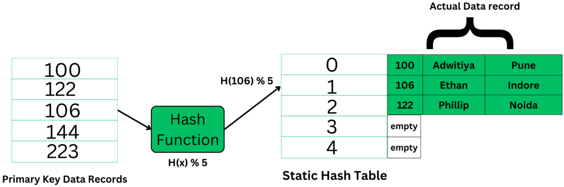
The primary key is used as the input to the hash function and the hash function generates the output as the hash index (bucket's address) which contains the address of the actual data record on the disk block.
Static Hashing has the following Properties
- Fixed Table Size: The number of buckets remains constant.
- Simple Hash Function: Typically uses a modulo function.
- Best for Known Data Size: Efficient when the number of records is known and stable.
- Inefficient with Dynamic Data: As data grows, collisions increase, leading to bucket overflows or skew.
To resolve this problem of bucket overflow, techniques such as - chaining and open addressing are used. Here's a brief info on both:
2. Chaining (Separate Chaining)
Chaining is a mechanism in which the hash table is implemented using an array of type nodes, where each bucket is of node type and can contain a long chain of linked lists to store the data records. So, even if a hash function generates the same value for any data record it can still be stored in a bucket by adding a new node.
Given:
- Hash table size = 5
- Hash function:
h(key) = key % 5 - Keys to insert: 10, 15, 20, 25, 30, 11
Step-by-step hashing:
| Key | Hash Index (key % 5) | Inserted At |
|---|---|---|
| 10 | 0 | Bucket 0 → [10] |
| 15 | 0 | Bucket 0 → [10 → 15] |
| 20 | 0 | Bucket 0 → [10 → 15 → 20] |
| 25 | 0 | Bucket 0 → [10 → 15 → 20 → 25] |
| 30 | 0 | Bucket 0 → [10 → 15 → 20 → 25 → 30] |
| 11 | 1 | Bucket 1 → [11] |
Final Hash Table (with separate chaining):
| Index | Linked List (Bucket) |
|---|---|
| 0 | 10 → 15 → 20 → 25 → 30 |
| 1 | 11 |
| 2 | -- |
| 3 | -- |
| 4 | -- |
Key Points:
- All keys that hash to the same index (like 10, 15, 20, etc.) are stored in a linked list at that index.
- Separate chaining avoids clustering and makes insertion easier.
- Efficient when hash table load factor is high.
However, this will give rise to the problem bucket skew that is, if the hash function keeps generating the same value again and again then the hashing will become inefficient as the remaining data buckets will stay unoccupied or store minimal data.
3. Open Addressing (Closed Hashing)
This is also called closed hashing this aims to solve the problem of collision by looking out for the next empty slot available which can store data. It uses techniques like linear probing, quadratic probing, double hashing, etc.
Example:
- Hash table size = 7
- Hash function:
h(key) = key % 7 - Collision resolution: Linear Probing
Insert the keys: 50, 700, 76, 85, 92, 73
Step-by-step insertion:
| Key | Hash (key % 7) | Insert At | Collision? | Final Position (after probing) |
|---|---|---|---|---|
| 50 | 50 % 7 = 1 | 1 | No | 1 |
| 700 | 700 % 7 = 0 | 0 | No | 0 |
| 76 | 76 % 7 = 6 | 6 | No | 6 |
| 85 | 85 % 7 = 1 | 1 | Yes | 2 (next slot) |
| 92 | 92 % 7 = 1 | 1 | Yes | 3 (after 1 and 2 are filled) |
| 73 | 73 % 7 = 3 | 3 | Yes | 4 (next slot after 3) |
Final Hash Table (index → value):
| Index | 0 | 1 | 2 | 3 | 4 | 5 | 6 |
|---|---|---|---|---|---|---|---|
| Value | 700 | 50 | 85 | 92 | 73 | -- | 76 |
4. Dynamic Hashing
Dynamic hashing is also known as extendible hashing, used to handle database that frequently changes data sets. This method offers us a way to add and remove data buckets on demand dynamically. This way as the number of data records varies, the buckets will also grow and shrink in size periodically whenever a change is made.
Properties of Dynamic Hashing
- Flexible Hash Function: Adapts based on data size.
- Directories: Point to buckets and may grow in size.
- Global Depth: Number of bits in directory indices.
- Bucket Splitting: Prevents overflow and ensures balanced distribution.
Working of Dynamic Hashing
Example: If global depth: k = 2, the keys will be mapped accordingly to the hash index. K bits starting from LSB will be taken to map a key to the buckets. That leaves us with the following 4 possibilities: 00, 11, 10, 01.

As we can see in the above image, the k bits from LSBs are taken in the hash index to map to their appropriate buckets through directory IDs. The hash indices point to the directories, and the k bits are taken from the directories' IDs and then mapped to the buckets. Each bucket holds the value corresponding to the IDs converted in binary.