Image classification is a fundamental task in computer vision where a model learns to identify and assign labels to images based on their visual content. It plays a key role in applications such as object recognition, facial detection, and autonomous systems. CIFAR‑10 image classification is a popular computer vision task that involves training models to recognize objects across ten distinct categories using the CIFAR‑10 dataset.
- Uses a standard benchmark dataset with 60,000 labelled images
- Commonly implemented with convolutional neural networks (CNNs)
- Ideal for learning and experimenting with deep learning in computer vision
Step-By-Step Implementation
Step 1: Import Libraries
- import tensorflow.keras for CNN layers and models
- import matplotlib.pyplot for visualisation
- to_categorical for one-hot encoding
import tensorflow as tf
from tensorflow.keras import datasets, layers, models
from tensorflow.keras.utils import to_categorical
import matplotlib.pyplot as plt
import numpy as np
Step 2: Load CIFAR-10 Dataset
- Training Set: 50,000 images
- Test Set: 10,000 images
- Classes: Airplane, Automobile, Bird, Cat, Deer, Dog, Frog, Horse, Ship, Truck
(X_train, y_train), (X_test, y_test) = datasets.cifar10.load_data()
Step 3: Preprocess Data
- Normalization scales pixel values to the range [0, 1], improving model stability and convergence.
- One-hot encoding converts each label into a 10-dimensional vector for multiclass classification.
X_train = X_train.astype('float32') / 255.0
X_test = X_test.astype('float32') / 255.0


y_train = to_categorical(y_train, 10)
y_test = to_categorical(y_test, 10)
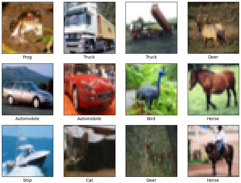
Step 4: Visualize Sample Images
- Displays a 4×4 grid of sample images from the training set.
- Each image is labeled with its corresponding class name.
class_names = ['Airplane','Automobile','Bird','Cat','Deer','Dog','Frog','Horse','Ship','Truck']

plt.figure(figsize=(10,10))
for i in range(16):
    plt.subplot(4,4,i+1)
    plt.xticks([])
    plt.yticks([])
    plt.grid(False)
    plt.imshow(X_train[i])
    plt.xlabel(class_names[np.argmax(y_train[i])])
plt.show()
Output:
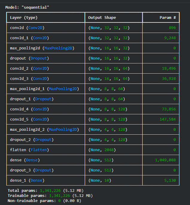
Step 5: Build the CNN Model
- Convolutional layers extract important spatial features from images.
- MaxPooling reduces the feature map size and computational load.
- Dropout helps prevent overfitting by randomly disabling neurons during training.
- Softmax layer produces probability scores for the 10 CIFAR-10 classes.
model = models.Sequential()


model.add(layers.Conv2D(32, (3,3), activation='relu', padding='same', input_shape=(32,32,3)))
model.add(layers.Conv2D(32, (3,3), activation='relu', padding='same'))
model.add(layers.MaxPooling2D((2,2)))
model.add(layers.Dropout(0.25))


model.add(layers.Conv2D(64, (3,3), activation='relu', padding='same'))
model.add(layers.Conv2D(64, (3,3), activation='relu', padding='same'))
model.add(layers.MaxPooling2D((2,2)))
model.add(layers.Dropout(0.25))


model.add(layers.Conv2D(128, (3,3), activation='relu', padding='same'))
model.add(layers.Conv2D(128, (3,3), activation='relu', padding='same'))
model.add(layers.MaxPooling2D((2,2)))
model.add(layers.Dropout(0.25))


model.add(layers.Flatten())
model.add(layers.Dense(512, activation='relu'))
model.add(layers.Dropout(0.5))
model.add(layers.Dense(10, activation='softmax'))
Step 6: Compile the Model
- Optimizer: Adam provides fast and stable convergence.
- Loss Function: Categorical cross-entropy is used for multiclass output.
- Metrics: Accuracy helps track model performance during training.
model.compile(optimizer='adam',
              loss='categorical_crossentropy',
              metrics=['accuracy'])

model.summary()
Output:
Step 7: Train the Model
- Epochs: 30 training cycles for learning patterns effectively.
- Batch Size: 64 samples per batch for efficient gradient updates.
- Validation Split: Helps monitor overfitting and generalization.
- History Object: Stores accuracy and loss values for later visualization.
history = model.fit(X_train, y_train,
                    epochs=30,
                    batch_size=64,
                    validation_split=0.2)
Step 8: Plot Training History
- Check for overfitting or underfitting
- Visual representation helps debug training issues
plt.figure(figsize=(12,5))


plt.subplot(1,2,1)
plt.plot(history.history['accuracy'], label='Train Accuracy')
plt.plot(history.history['val_accuracy'], label='Validation Accuracy')
plt.title('Model Accuracy')
plt.xlabel('Epoch')
plt.ylabel('Accuracy')
plt.legend()


plt.subplot(1,2,2)
plt.plot(history.history['loss'], label='Train Loss')
plt.plot(history.history['val_loss'], label='Validation Loss')
plt.title('Model Loss')
plt.xlabel('Epoch')
plt.ylabel('Loss')
plt.legend()

plt.show()
Output:
Model Accuracy Graph:
- The training accuracy increases steadily with each epoch, showing that the model is learning patterns from the data.
- Validation accuracy also improves but starts to level off after some epochs.
- The small gap between training and validation accuracy suggests the model generalizes reasonably well, with only mild overfitting toward the end.
Model Loss Graph:
- Training loss consistently decreases, meaning the model’s predictions are getting better on training data.
- Validation loss drops initially but then fluctuates slightly, indicating that learning has stabilized.
- This behavior shows the model has mostly converged, and further training may not give significant improvement.
Step 10: Predict on Test Images
- Use model.predict to get class probabilities
- Display predicted and true labels
def plot_predictions(index):
    img = X_test[index]
    true_label = class_names[np.argmax(y_test[index])]
    pred_probs = model.predict(np.expand_dims(img, axis=0))
    pred_label = class_names[np.argmax(pred_probs)]

    plt.imshow(img)
    plt.title(f"True: {true_label} | Pred: {pred_label}")
    plt.axis('off')
    plt.show()


for i in range(5):
    plot_predictions(i)
Output:
We can see our model is working fine.
You can download full code from here.