

Classification means grouping things into categories based on their similarities or characteristics. A Perceptron is a neural network that makes decisions by combining inputs with weights and applying an activation function. Classification with Perceptron shows how simple linear decision boundaries separate data into meaningful classes using iterative weight updates.
Mathematical Intuition
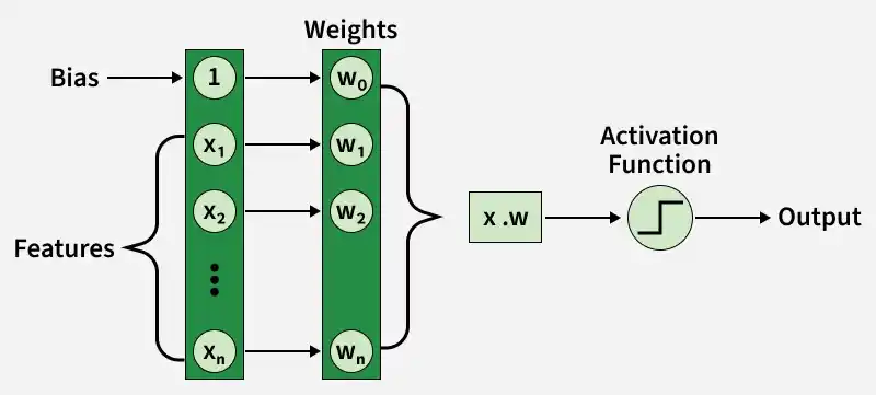
The Perceptron makes decisions by computing a weighted sum of its inputs and applying an activation function to produce an output. Mathematically, this is expressed as:
z = w_1 x_1 + w_2 x_2 + \cdots + w_n x_n + b
where
x_{i} are input featuresw_{i} are the corresponding weights.- b is the bias term that shifts the decision boundary
The weighted sum
Activation Function
An activation function is a mathematical function that determines a neuron’s output by transforming the weighted sum of inputs. It introduces non-linearity and allows the Perceptron to make decisions.
Sigmoid Function
Sigmoid is a type of activation function and is commonly used in binary classification because it maps any input to a value between 0 and 1, allowing us to interpret the result as a probability.
\sigma(z) = \frac{1}{1 + e^{-z}}
Once the weighted sum z passes through the activation function, the final Perceptron output y is computed as:
y=f(z)
f(z) can be a step function, sigmoid or other activation.- The output
y represents the predicted class of the input.
This output is used to calculate error and iteratively update weights, enabling the Perceptron to separate data with a linear boundary.
Loss Function for Classification
In binary classification the loss function measures how far the predicted output is from the actual target value. It helps quantify the error of the model and guides the weight update process during training.
L(y, \hat{y}) = -\big[y\log(\hat{y}) + (1 - y)\log(1 - \hat{y})\big]
y : Actual target label\hat{y} : Predicted probability\log(\hat{y}) : Penalizes wrong confident predictions for class 1\log(1-\hat{y}) : Penalizes wrong confident predictions for class 0
Why Cross-Entropy Loss
- If the prediction is correct, the loss is 0
- If the prediction is wrong, the loss becomes very large
- Incorrect confident predictions are heavily penalized
Computing Gradients of the Loss Function
To train the Perceptron for classification, we need to minimize the Binary Cross-Entropy loss. This is done by computing the gradients of the loss with respect to the weights and bias. Gradients tell us how much each parameter should change to reduce the error.
1. Gradient with respect to Weights: We compute the gradient with respect to each weight to determine how much that weight contributes to the overall loss.
\frac{\partial L}{\partial w_{i}} = (\hat{y} - y)x_{i}
2. Gradient with respect to Bias: The gradient with respect to the bias measures how the loss changes when the bias term is adjusted.
\frac{\partial L}{\partial b} = (\hat{y} - y)
Gradient Descent Optimization
Gradient Descent Optimization is an iterative method used to minimize a loss function by updating model parameters using gradients. It updates weights and bias in the direction opposite to the gradient to reduce error.
w_{i} = w_{i} - \alpha \frac{\partial L}{\partial w_{i}}
b = b - \alpha \frac{\partial L}{\partial b}
Here,
Step-By-Step Implementation
Step 1: Import Libraries
Here we import:
- NumPy for numerical computations
- Pandas for data handling
- Scikit-learn for preprocessing and splitting the dataset
- Matplotlib for visualization
import numpy as np
import pandas as pd
from sklearn.model_selection import train_test_split
from sklearn.preprocessing import StandardScaler
import matplotlib.pyplot as plt
Step 2: Loading the Dataset
Load the Titanic dataset into a pandas DataFrame.
You can download full code from here
df = pd.read_csv('/content/Titanic-Dataset.csv')
Step 3: Data Preprocessing
Select relevant features, handle missing values and convert categorical variables to numeric.
df = df[["Survived", "Pclass", "Sex", "Age", "Fare", "SibSp", "Parch", "Embarked"]]
df["Age"].fillna(df["Age"].median(), inplace=True)
df["Embarked"].fillna(df["Embarked"].mode()[0], inplace=True)
df["Sex"] = df["Sex"].map({"male": 0, "female": 1})
df = pd.get_dummies(df, columns=["Embarked"], drop_first=True)
Step 4: Split Input and Target, Scale Features
Separate features and target variable, then scale features for better gradient descent performance.
X = df.drop("Survived", axis=1).values
y = df["Survived"].values.reshape(-1, 1)

scaler = StandardScaler()
X = scaler.fit_transform(X)

X_train, X_test, y_train, y_test = train_test_split(X, y, test_size=0.2, random_state=42)
Step 5: Define Sigmoid Activation Function
The sigmoid function maps net input values to probabilities between 0 and 1.
def sigmoid(z):
    return 1 / (1 + np.exp(-z))
Step 6: Define Cross-Entropy Loss Function
Cross-entropy loss measures the difference between predicted probabilities and true labels.
def compute_loss(y, y_hat):
    m = y.shape[0]
    loss = - (1/m) * np.sum(y * np.log(y_hat) + (1 - y) * np.log(1 - y_hat))
    return loss
Step 7: Initialize Parameters
Randomly initialize weights and bias, set learning rate and number of epochs.
n_features = X_train.shape[1]
W = np.random.randn(n_features, 1) * 0.01
b = 0.0
learning_rate = 0.01
epochs = 2000
Step 8: Train Perceptron using Gradient Descent
Iteratively compute predictions, calculate loss, compute gradients and update parameters.
loss_history = []

for epoch in range(epochs):
    z = np.dot(X_train, W) + b
    y_hat = sigmoid(z)

    loss = compute_loss(y_train, y_hat)
    loss_history.append(loss)

    dz = y_hat - y_train
    dW = (1/X_train.shape[0]) * np.dot(X_train.T, dz)
    db = (1/X_train.shape[0]) * np.sum(dz)

    W -= learning_rate * dW
    b -= learning_rate * db

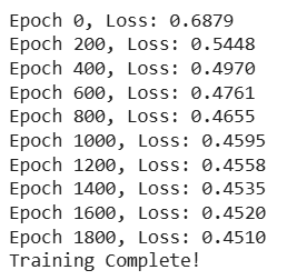
    if epoch % 200 == 0:
        print(f"Epoch {epoch}, Loss: {loss:.4f}")
Output:
Step 9: Evaluate Model on Test Set
Compute predictions on the test set and calculate accuracy.
z_test = np.dot(X_test, W) + b
y_hat_test = sigmoid(z_test)
y_pred = (y_hat_test > 0.5).astype(int)

accuracy = np.mean(y_pred == y_test) * 100
print(f"\nTest Accuracy: {accuracy:.2f}%")
Output:
Test Accuracy: 78.77%
Step 10: Plot Training Loss
Visualize how the cross-entropy loss decreases over epochs.
plt.plot(loss_history)
plt.title("Training Loss (Cross-Entropy)")
plt.xlabel("Epochs")
plt.ylabel("Loss")
plt.show()
Output:
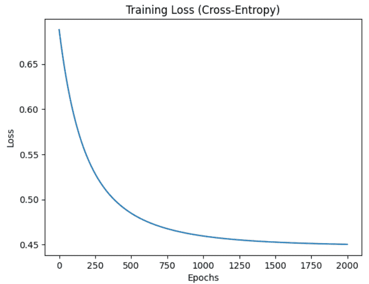
Here we can see training loss is reducing hence model is working fine.
You can download full code from here