Time Series Forecasting using TensorFlow

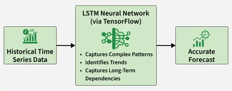
TensorFlow is a framework that enables us to apply deep learning techniques to time series analysis. By using neural networks, we can capture complex patterns, trends and long-term dependencies in sequential data, leading to more accurate forecasts. Here, we will explore how LSTM models can be used for time series forecasting.

Here we will do:

• Time Series Analysis: Start by understanding data collected over time and identifying patterns like trends and seasonality.
• Deep Learning Approach: Use neural networks to automatically learn complex temporal relationships from historical data.
• TensorFlow Framework: Build and train our deep learning model using TensorFlow.
• LSTM Model: Implement an LSTM network designed to handle sequence data and long-term dependencies.
• Forecasting: Use the trained model to predict future values based on past data.

Why LSTM for Time Series Forecasting?

Long Short Term Memory (LSTM) is an advanced type of Recurrent Neural Network (RNN) built to handle the limitations of traditional RNNs. Standard RNNs often face the vanishing or exploding gradient problem, which weakens their ability to retain information across long sequences. LSTM overcomes this through a dedicated memory cell (cell state) that selectively stores and updates information over time.

• Stable Training: Gated architecture controls information flow, preventing gradient instability during backpropagation.
• Captures Long Term Patterns: Effectively models trends, seasonality and delayed effects in time dependent data.
• Handles Non Linearity: Learns complex, non linear relationships that frequently exist in real world datasets.
• Supports Variable Length Sequences: Works seamlessly with sequences of different sizes without architectural changes.
• Implicit Feature Extraction: Automatically derives meaningful temporal features directly from raw input data.

Implementation

We will use Air Passengers dataset to demonstrate univariate time series forecasting with an LSTM model. This dataset contains monthly passenger numbers for flights within the United States from 1949 to 1960.

Step 1: Load and Visualize the Dataset

• Necessary libraries like Numpy, Pandas, Matplotlib, Scikit learn and Tensorflow are imported.
• Data processing has been done by converting the Month column to datetime format using pd.to_datetime().
• We set the Month column as the index of the DataFrame using set_index().

You can download dataset from here

import numpy as np
import pandas as pd
import matplotlib.pyplot as plt
from sklearn.preprocessing import MinMaxScaler
from tensorflow.keras.models import Sequential
from tensorflow.keras.layers import LSTM, Dense

data = pd.read_csv("AirPassengers.csv")

data['Month'] = pd.to_datetime(data['Month'])

data.set_index('Month', inplace=True)

data.head()

Output:

The dataset records the data of the passenger on the first day of every month starting from 1949 to 1960.

plt.figure(figsize=(10, 6))
plt.plot(data)
plt.title('Air Passengers Time Series')
plt.xlabel('Year')
plt.ylabel('Number of Passengers')
plt.show()

Output:

The line graph is showing clear upward trend in the number of passengers over time. This suggests that air travel was becoming more popular during this period.

Step 2: Preprocessing the Data

Feature scaling is essential for neural network models to ensure that all input features are within a similar range, preventing any particular feature from dominating the learning process due to its scale.

scaler = MinMaxScaler()
scaled_data = scaler.fit_transform(data)

train_size = int(len(scaled_data) * 0.8)
train_data = scaled_data[:train_size]
test_data = scaled_data[train_size:]

Step 3: Creating Sequences for LSTM Model

Now, let's create sequences of input data and corresponding target values for training the LSTM model:

• create_sequences() takes two inputs i.e the time series data and seq_length (number of past time steps to consider).
• We go through the data and for each step, take seq_length previous values as input (X) and the next value as the target (y).
• The function returns NumPy arrays X (input sequences) and y (target values), and we use it to create sequences for both training and testing datasets.

def create_sequences(data, seq_length):
    X, y = [], []
    for i in range(len(data) - seq_length):
        X.append(data[i:i+seq_length])
        y.append(data[i+seq_length])
    return np.array(X), np.array(y)

seq_length = 12  
X_train, y_train = create_sequences(train_data, seq_length)
X_test, y_test = create_sequences(test_data, seq_length)

Step 4: Defining and Training the LSTM Model

Now, let's define and train the LSTM model:

• We create a model using Sequential() and add an LSTM layer with 50 units, ReLU activation and input shape (seq_length, 1) so it can learn from sequence data.
• We add a Dense layer with 1 unit to output the predicted value (since this is a regression problem).
• Finally, we compile the model using the Adam optimizer and mean squared error (MSE) loss function and then train it on the training data.

model = Sequential([
    LSTM(50, activation='relu', input_shape=(seq_length, 1)),
    Dense(1)
])

model.compile(optimizer='adam', loss='mse')
model.fit(X_train, y_train, epochs=100, batch_size=32, verbose=1)

Output:

Step 5: Predictions and Visualization

Finally, let's make predictions using the trained model and evaluate its performance and understanding the plot of actual data points and a forecasted trendline.

train_predictions = model.predict(X_train)
test_predictions = model.predict(X_test)

train_predictions = scaler.inverse_transform(train_predictions)
test_predictions = scaler.inverse_transform(test_predictions)

plt.figure(figsize=(10, 6))

plt.plot(data.index[seq_length:], data['#Passengers'][seq_length:], label='Actual', color='blue')

plt.plot(data.index[seq_length:seq_length+len(train_predictions)], train_predictions, label='Train Predictions',color='green')

test_pred_index = range(seq_length+len(train_predictions), seq_length+len(train_predictions)+len(test_predictions))
plt.plot(data.index[test_pred_index], test_predictions, label='Test Predictions',color='orange')

plt.title('Air Passengers Time Series Forecasting')
plt.xlabel('Year')
plt.ylabel('Number of Passengers')
plt.legend()
plt.show()

Output:

Step 6: Forecasting

In this model, to understand the forecasting precisely, let's create a graph for the period of 30 days:

• Initialize an empty list to store the forecasted values, we use the last sequence from the test data to initialize last_sequence with a loop through the forecast period to predict the next value using the model.
• Let's plot the actual values for the test period along with the forecasted values for the next 30 days.

forecast_period = 30
forecast = []

last_sequence = X_test[-1]

for _ in range(forecast_period):
    current_sequence = last_sequence.reshape(1, seq_length, 1)
    next_prediction = model.predict(current_sequence)[0][0]
    forecast.append(next_prediction)
    last_sequence = np.append(last_sequence[1:], next_prediction)

forecast = scaler.inverse_transform(np.array(forecast).reshape(-1, 1))

plt.figure(figsize=(10, 6))
plt.plot(data.index[-len(test_data):], scaler.inverse_transform(test_data), label='Actual')
plt.plot(pd.date_range(start=data.index[-1], periods=forecast_period, freq='M'), forecast, label='Forecast')
plt.title('Air Passengers Time Series Forecasting (30-day Forecast)')
plt.xlabel('Year')
plt.ylabel('Number of Passengers')
plt.legend()
plt.show()

Output:

The forecast represents passenger numbers for the next 30 months, not 30 days, since the dataset is monthly. Both actual and predicted values show an overall upward trend. The actual data has clear seasonal peaks and the forecast captures this pattern, though in a smoother form.

Download full code from here