Recurrent Neural Networks (RNNs) are neural networks designed to process sequential data by maintaining hidden states that store information from previous steps. In this implementation, TensorFlow is used to build and train an RNN model for sequence learning tasks.
Implementation
1. Importing Libraries
We will be importing Pandas, NumPy, Matplotlib, Seaborn, TensorFlow, Keras, NLTK and Scikit-learn for implementation.
import warnings
from tensorflow.keras.utils import pad_sequences
from tensorflow.keras.preprocessing.text import Tokenizer
from sklearn.model_selection import train_test_split
import tensorflow as tf
from tensorflow import keras
import pandas as pd
import matplotlib.pyplot as plt
import seaborn as sns
import plotly.express as px
import numpy as np

import re
import nltk
nltk.download('all')
from nltk.corpus import stopwords
from nltk.tokenize import word_tokenize
from nltk.stem import WordNetLemmatizer
lemm = WordNetLemmatizer()

warnings.filterwarnings("ignore")
2. Loading the Dataset
The dataset is loaded using pd.read_csv() and cleaned by removing rows with null values in the Class Name column.
- Loads dataset using Pandas
- Displays first 7 rows using data.head(7)
- Removes null values from Class Name column
data = pd.read_csv("Clothing Review.csv")
data.head(7)

data = data[data['Class Name'].isnull() == False]
Output:

3. Performing Exploratory Data Analysis
EDA helps understand the distribution and patterns in the dataset before building the model using different visualization techniques.
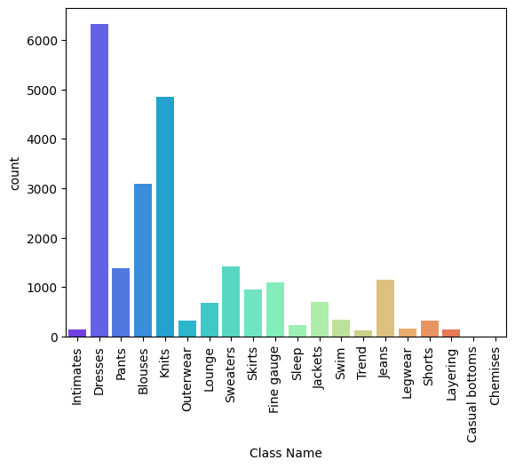
Count Plot of Class Name Distribution
sns.countplot() is used to visualize the count of each category in the Class Name column. The x-axis labels are rotated using plt.xticks(rotation=90) for better readability.
sns.countplot(data=data, x='Class Name', palette='rainbow')
plt.xticks(rotation=90)
plt.show()
Output:
Count Plot of Rating and Recommendation Distribution
A figure of size 12×5 is created using plt.subplots() to visualize the distribution of ratings and recommendation indicators.
plt.subplots(figsize=(12, 5))
plt.subplot(1, 2, 1)
sns.countplot(data=data, x='Rating',palette="deep")

plt.subplot(1, 2, 2)
sns.countplot(data=data, x="Recommended IND", palette="deep")
plt.show()
Output:

Histogram of Age Distribution
A histogram is created using px.histogram() to visualize the frequency distribution of age. The plot also includes a box plot to show spread and outliers.
fig = px.histogram(data, marginal='box',
                   x="Age", title="Age Group",
                   color="Recommended IND",
                   nbins=65-18,
                   color_discrete_sequence=['green', 'red'])
fig.update_layout(bargap=0.2)
Output:

Interpretation of Age Distribution Plot
The histogram shows age distribution for recommended and non-recommended individuals, while the box plots display the spread and outliers for each group.
- Green bars represent recommended individuals
- Red bars represent non-recommended individuals
- Box plots show spread and outliers of age values
- Helps compare age distribution between groups
- Can also be used to analyze age distribution with ratings
fig = px.histogram(data,
                   x="Age",
                   marginal='box',
                   title="Age Group",
                   color="Rating",
                   nbins=65-18,
                   color_discrete_sequence
                   =['black', 'green', 'blue', 'red', 'yellow'])
fig.update_layout(bargap=0.2)
Output:

4. Prepare the Data to build Model
Since the dataset is NLP-based, text columns are used as features and the Rating column is used for sentiment analysis. To handle class imbalance, ratings above 3 are converted to 1 (positive) and ratings below 3 are converted to 0 (negative).
- Uses text columns as input features
- Uses Rating column for sentiment analysis
- Handles imbalance in rating distribution
- Converts ratings >3 to positive class (1)
- Converts ratings <3 to negative class (0)
def filter_score(rating):
    return int(rating > 3)

features = ['Class Name', 'Title', 'Review Text']

X = data[features]
y = data['Rating']
y = y.apply(filter_score)
5. Text Preprocessing
Text preprocessing is performed to clean and standardize the text data before training the model. The text is converted to lowercase, lemmatized and cleaned by removing stopwords and punctuation.
- Converts text to lowercase for consistency
- Applies lemmatization to normalize words
- Removes stopwords and punctuation
- Reduces noise and improves text quality for training
def toLower(data):
    if isinstance(data, float):
        return '<UNK>'
    else:
        return data.lower()

stop_words = stopwords.words("english")

def remove_stopwords(text):
    no_stop = []
    for word in text.split(' '):
        if word not in stop_words:
            no_stop.append(word)
    return " ".join(no_stop)

def remove_punctuation_func(text):
    return re.sub(r'[^a-zA-Z0-9]', ' ', text)

X['Title'] = X['Title'].apply(toLower)
X['Review Text'] = X['Review Text'].apply(toLower)

X['Title'] = X['Title'].apply(remove_stopwords)
X['Review Text'] = X['Review Text'].apply(remove_stopwords)

X['Title'] = X['Title'].apply(lambda x: lemm.lemmatize(x))
X['Review Text'] = X['Review Text'].apply(lambda x: lemm.lemmatize(x))

X['Title'] = X['Title'].apply(remove_punctuation_func)
X['Review Text'] = X['Review Text'].apply(remove_punctuation_func)

X['Text'] = list(X['Title']+X['Review Text']+X['Class Name'])


X_train, X_test, y_train, y_test = train_test_split(
    X['Text'], y, test_size=0.25, random_state=42)
6. Tokenization
Tokenization converts text data into numerical vectors that can be processed by the neural network. Keras provides a Tokenizer API to create word indices from the text data.
- Converts text into numerical sequences
- Uses Keras Tokenizer for preprocessing
- num_words defines vocabulary size
- OOV handles out-of-vocabulary words
- fit_on_texts() is applied only on training data
tokenizer = Tokenizer(num_words=10000, oov_token='<OOV>')
tokenizer.fit_on_texts(X_train)
7. Padding the Text Data
Padding is used to make all text sequences the same length before feeding them into the neural network. Extra zeros are added to shorter sequences, while longer sequences can be truncated if needed.
- Makes all text sequences equal in length
- Adds zeros to shorter sequences
- Longer sequences can be truncated
- Padding and tokenization are general NLP preprocessing techniques
- Helps in efficient training of neural network models
train_seq = tokenizer.texts_to_sequences(X_train)
test_seq = tokenizer.texts_to_sequences(X_test)

train_pad = pad_sequences(train_seq,
                          maxlen=40,
                          truncating="post",
                          padding="post")
test_pad = pad_sequences(test_seq,
                         maxlen=40,
                         truncating="post",
                         padding="post")
8. Building a Recurrent Neural Network (RNN) in TensorFlow
After preprocessing the data, a Simple Recurrent Neural Network (SimpleRNN) is built for training. Before entering the RNN layer, the text data is passed through an Embedding layer to generate fixed-size word vectors.
- Builds a SimpleRNN model using TensorFlow
- Uses an Embedding layer before the RNN layer
- Embedding converts words into dense vector representations
- Fixed-size vectors help improve sequence learning
from tensorflow import keras

model = keras.models.Sequential()
model.add(keras.layers.Embedding(input_dim=10000, output_dim=128, input_length=40))
model.add(keras.layers.SimpleRNN(64, return_sequences=True))
model.add(keras.layers.SimpleRNN(64))
model.add(keras.layers.Dense(128, activation="relu"))
model.add(keras.layers.Dropout(0.4))
model.add(keras.layers.Dense(1, activation="sigmoid"))

model.build(input_shape=(None, 40))

model.summary()
Output:

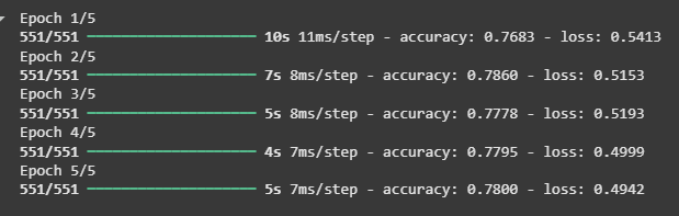
9. Training the Model
After building the model, it is compiled using an optimizer, loss function and evaluation metric. The model is then trained on the preprocessed training data for multiple epochs.
- Compiles model using optimizer, loss function and evaluation metric
- Trains the model on train_pad data
- Uses y_train as target labels
- Runs training for 5 epochs to evaluate accuracy
model.compile(loss="binary_crossentropy",
              optimizer="adam",
              metrics=["accuracy"])


history = model.fit(train_pad,
                    y_train,
                    epochs=5)
Output:
Download full code from here