Association rules are a fundamental concept used to find relationships, correlations or patterns within large sets of data items. They describe how often itemsets occur together in transactions and express implications of the form:

X \rightarrow Y

Where X and Y are disjoint sets of items. This rule suggests that when items in X appear, items in Y tend to appear as well. Association rules originated from market basket analysis and help retailers and analysts understand customer behavior by discovering item associations in transaction data. For example, a rule stating

\{ \text{Bread}, \text{Butter} \} \;\rightarrow\; \{ \text{Milk} \}

Indicates that customers who buy bread and butter also tend to buy milk.

Key Components

• Antecedent (X): The "if" part representing one or more items found in transactions.
• Consequent (Y): The "then" part, representing the items likely to be purchased when antecedent items appear.

Rules are evaluated based on metrics that quantify their strength and usefulness:

Rule Evaluation Metrics

1. Support: Fraction of transactions containing the itemsets in both X and Y.

\text{Support}(X \rightarrow Y) = \frac{\text{Number of transactions with } (X \cup Y)}{\text{Total number of transactions}}

Support measures how frequently the combination appears in the data.

2. Confidence: Probability that transactions with X also include Y.

\text{Confidence}(X \rightarrow Y) = \frac{\text{Support}(X \cup Y)}{\text{Support}(X)}

Confidence measures the reliability of the inference.

3. Lift: The ratio of observed support to that expected if X and Y were independent.

\text{Lift}(X \rightarrow Y) = \frac{\text{Confidence}(X \rightarrow Y)}{\text{Support}(Y)}

• Lift > 1 implies a positive association — items occur together more than expected.
• Lift = 1 implies independence.
• Lift < 1 implies a negative association.

Example Transaction Data

Considering the rule:

\{ \text{Milk}, \text{Diaper} \} \;\rightarrow\; \{ \text{Beer} \}

Calculations:

• Support =\frac 2 5 = 0.4
• Confidence = \frac 2 3 \approx 0.67
• Lift = \frac{0.67}{0.6} = 1.11 (positive association)

Implementation

Let's see the working,

Step 1: Install and Import Libraries

We will install and import all the required libraries such as pandas, mixtend, matplotlib, networkx.

!pip install pandas mlxtend matplotlib seaborn networkx

import pandas as pd
from mlxtend.preprocessing import TransactionEncoder
from mlxtend.frequent_patterns import apriori, association_rules
import matplotlib.pyplot as plt
import seaborn as sns
import networkx as nx

Step 2: Load and Preview Dataset

We will upload the dataset,

data = pd.read_csv("Groceries_dataset.csv")

print(data.head())

Output:

Step 3: Prepare Data for Apriori Algorithm

Apriori requires this one-hot encoded format where columns = items and rows = transactions with True/False flags.

transactions = data.groupby('Member_number')[
    'itemDescription'].apply(list).values.tolist()

te = TransactionEncoder()
te_ary = te.fit(transactions).transform(transactions)
df = pd.DataFrame(te_ary, columns=te.columns_)
df.head()

Output:

Step 4: Generate Frequent Itemsets

We will,

• Finds itemsets appearing in ≥ 1% of all transactions.
• use_colnames=True to keep item names readable.

frequent_itemsets = apriori(df, min_support=0.01, use_colnames=True)

print(frequent_itemsets.head())

Output:

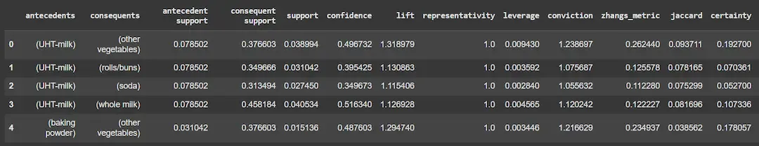
Step 5: Generate Association Rules

We will,

• Extract rules with confidence ≥ 30%.
• Rules DataFrame includes columns like antecedents, consequents, support, confidence and lift.

rules = association_rules(
    frequent_itemsets, metric="confidence", min_threshold=0.3)

print(rules.head())

Output:

Step 6: Visualize Top Frequent Items

We will,

• Visualizes the 10 most purchased items.
• Helps understand popular products in the dataset.

item_frequencies = df.sum().sort_values(ascending=False)

plt.figure(figsize=(10, 6))
sns.barplot(x=item_frequencies.head(10).values,
            y=item_frequencies.head(10).index)
plt.title('Top 10 Frequent Items')
plt.xlabel('Frequency')
plt.ylabel('Items')
plt.show()

Output:

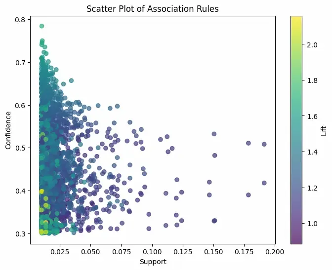
Step 7: Scatter Plot of Rules(Support vs Confidence)

Here we will,

• Shows the relationship between support and confidence for rules.
• Color encodes the strength of rules via lift.

plt.figure(figsize=(8, 6))
scatter = plt.scatter(rules['support'], rules['confidence'],
                      c=rules['lift'], cmap='viridis', alpha=0.7)
plt.colorbar(scatter, label='Lift')
plt.xlabel('Support')
plt.ylabel('Confidence')
plt.title('Scatter Plot of Association Rules')
plt.show()

Output:

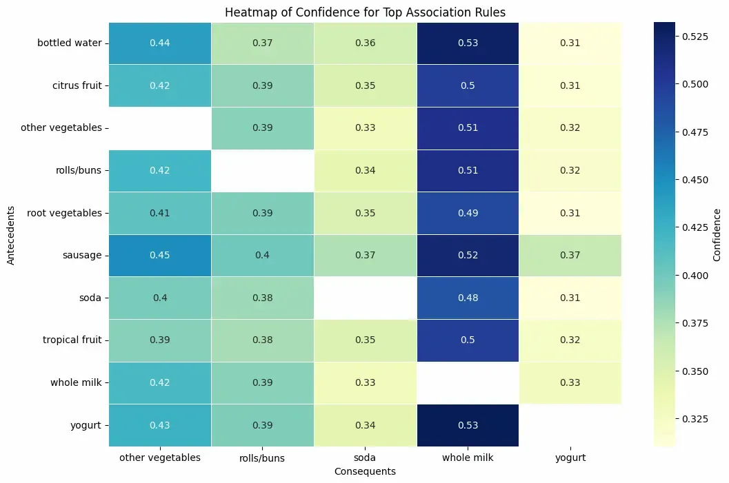
Step 8: Heatmap of Confidence for Selected Rules

We will,

• Shows confidence values between top antecedent and consequent itemsets.
• A quick way to identify highly confident rules.

rules['antecedents_str'] = rules['antecedents'].apply(
    lambda x: ', '.join(list(x)))
rules['consequents_str'] = rules['consequents'].apply(
    lambda x: ', '.join(list(x)))

top_ants = rules.groupby('antecedents_str')['support'].sum().nlargest(10).index
top_cons = rules.groupby('consequents_str')['support'].sum().nlargest(10).index

filtered = rules[(rules['antecedents_str'].isin(top_ants)) &
                 (rules['consequents_str'].isin(top_cons))]

heatmap_data = filtered.pivot(
    index='antecedents_str', columns='consequents_str', values='confidence')

plt.figure(figsize=(12, 8))
sns.heatmap(heatmap_data, annot=True, cmap='YlGnBu',
            linewidths=0.5, cbar_kws={'label': 'Confidence'})
plt.title('Heatmap of Confidence for Top Association Rules')
plt.xlabel('Consequents')
plt.ylabel('Antecedents')
plt.show()

Output:

Use Cases

Let's see the use case of Association rule,

• Market Basket Analysis: Identifies products often bought together to improve store layouts and promotions (e.g., bread and butter).
• Recommendation Systems: Suggests related items based on buying patterns (e.g., accessories with laptops).
• Fraud Detection: Detects unusual transaction patterns indicating fraud.
• Healthcare Analytics: Finds links between symptoms, diseases and treatments (e.g., symptom combinations predicting a disease).

Advantages

• Interpretable and Easy to Explain: Rules offer clear “if-then” relationships understandable to non-technical stakeholders.
• Unsupervised Learning: Works well on unlabeled data to find hidden patterns without prior knowledge.
• Flexible Data Types: Effective on transactional, categorical and binary data.
• Helps in Feature Engineering: Can be used to create new features for downstream supervised models.

Limitations

• Large Number of Rules: Can generate many rules, including trivial or redundant ones, making interpretation hard.
• Support Threshold Sensitivity: High support thresholds miss interesting but infrequent patterns; low thresholds generate too many rules.
• Not Suitable for Continuous Variables: Requires discretization or binning before use with numerical attributes.
• Computationally Expensive: Performance degrades on very large or dense datasets due to combinatorial explosion.
• Statistical Significance: High confidence doesn’t guarantee a meaningful rule; domain knowledge is essential to validate findings.