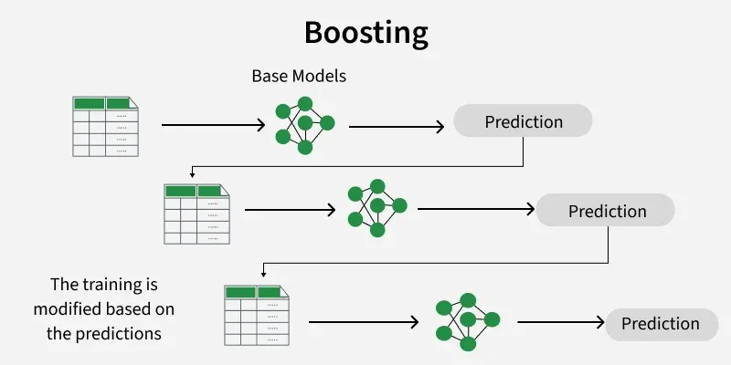
Boosting is an ensemble learning technique that improves predictive accuracy by combining multiple weak learners into a single strong model. It works iteratively where each new model focuses on correcting the mistakes of its predecessors and gradually improves overall performance.
- Trains models sequentially, with each learner improving upon the errors of the previous one.
- Assigns higher importance to hard-to-classify data points, ensuring difficult cases get more focus.
- Combines multiple weak learners using weighted aggregation to form a highly accurate strong model.
How Boosting Works
The process focuses on sequentially reducing errors by emphasising data points that are harder to classify. By iteratively refining predictions, boosting improves overall model accuracy.
1. Initialize Weights
All training instances are initially assigned equal weights to represent their importance. These weights determine how much influence each data point has on the first weak learner.
2. Sequential Training
- Train the first weak learner on the weighted dataset.
- Evaluate its predictions and identify misclassified instances.
- Increase the weights of misclassified examples so that the next learner focuses more on these harder cases.
3. Iterative Refinement
This process is repeated for multiple rounds. Each new weak learner is trained on the updated weighted data, addressing the mistakes of the existing ensemble. Over iterations the ensemble gradually improves its predictive performance.
4. Aggregate Predictions
The outputs of all weak learners are combined to produce the final prediction. Aggregation is typically done using weighted voting or averaging where models with higher accuracy have more influence on the final decision.
Types of Boosting Algorithms
Boosting methods differ in how they handle errors and combine weak learners to create a strong predictive model.
1. AdaBoost (Adaptive Boosting)
AdaBoost assigns higher weights to misclassified data points after each iteration, forcing subsequent learners to focus on harder cases. It is particularly effective for binary classification problems.
2. Gradient Boosting
Gradient Boosting trains each new model on the residual errors of the previous ensemble, using gradient descent to minimize the loss function. It can be applied to both regression and classification tasks.
3. XGBoost (Extreme Gradient Boosting)
XGBoost is an optimized scalable implementation of gradient boosting that supports parallel computation, regularization and handles large datasets efficiently, making it highly effective for practical machine learning problems.
Step By Step Implementation
Here we implement Adaboost Boosting Algorithm.
Step 1: Import Libraries
We import all necessary libraries such as numpy, pandas and scikit learn for data handling, preprocessing, model training and evaluation.
import pandas as pd
import numpy as np
from sklearn.model_selection import train_test_split
from sklearn.impute import SimpleImputer
from sklearn.preprocessing import LabelEncoder
from sklearn.tree import DecisionTreeClassifier
from sklearn.ensemble import AdaBoostClassifier
from sklearn.metrics import accuracy_score
Step 2: Load the Titanic Dataset
Load the Titanic CSV dataset and separate the features (X) from the target variable (y).
You can download dataset from here
titanic = pd.read_csv('Titanic-Dataset.csv')
X = titanic.drop(['PassengerId', 'Name', 'Ticket', 'Cabin', 'Survived'], axis=1)
y = titanic['Survived']
Step 3: Handle Missing Values
Impute missing numeric columns with the median and categorical columns with the most frequent value.
num_cols = X.select_dtypes(include=np.number).columns
cat_cols = X.select_dtypes(include='object').columns

imputer_num = SimpleImputer(strategy='median')
X[num_cols] = imputer_num.fit_transform(X[num_cols])

imputer_cat = SimpleImputer(strategy='most_frequent')
X[cat_cols] = imputer_cat.fit_transform(X[cat_cols])
Step 4: Encode Categorical Variables
Convert categorical features into numeric labels so they can be used by the model.
for col in cat_cols:
    le = LabelEncoder()
    X[col] = le.fit_transform(X[col])
Step 5: Split the Dataset
Split the dataset into training and testing sets.
X_train, X_test, y_train, y_test = train_test_split(
    X, y, test_size=0.2, random_state=42
)
Step 6: Train a Weak Learner (Decision Tree)
Train a simple decision tree with limited depth to act as the weak learner for AdaBoost.
weak_tree = DecisionTreeClassifier(max_depth=4, random_state=42)
weak_tree.fit(X_train, y_train)
Step 7: Train AdaBoost Classifier
Use AdaBoost to combine multiple weak learners into a strong model.
ada_boost = AdaBoostClassifier(
    estimator=weak_tree,
    n_estimators=100,
    learning_rate=1.0,
    random_state=42
)
ada_boost.fit(X_train, y_train)
Step 8: Evaluate Models
Compare the accuracy of the weak learner and the AdaBoost model on the test set.
tree_accuracy = accuracy_score(y_test, weak_tree.predict(X_test))
print(f'Accuracy of the weak learner (Decision Tree): {tree_accuracy*100:.2f}%')

ada_accuracy = accuracy_score(y_test, ada_boost.predict(X_test))
print(f'Accuracy of AdaBoost model: {ada_accuracy*100:.2f}%')
Output:
Accuracy of the weak learner (Decision Tree): 79.89%
Accuracy of AdaBoost model: 81.56%
You can download full code from here
Bagging vs Boosting
Bagging and boosting are both ensemble learning techniques, but they differ in how models are trained, how errors are handled and their impact on bias and variance.
Features | Boosting | Bagging |
|---|---|---|
Core Idea | Sequentially builds models that focus on correcting errors of previous models | Trains models independently on random data subsets and combines their predictions |
Objective | Improve accuracy by focusing on hard-to-classify instances | Stabilize predictions and prevent overfitting by averaging multiple models |
Model Training | Each model learns from the mistakes of its predecessor. | Models are trained independently on random samples and combined to improve stability |
Error Reduction | Reduces bias with some reduction in variance | Primarily reduces variance, especially useful for high-variance models |
Sensitivity to Outliers | More sensitive, as misclassified points receive higher weight | Less sensitive, since random sampling dilutes the impact of outliers |
Prediction Aggregation | Weighted voting or averaging | Simple majority voting or averaging of all models |
Advantages
- Reduces Bias: Sequentially combines weak learners to improve predictions, helping reduce high bias in simple models.
- Focus on Hard Cases: Gives higher importance to misclassified or difficult instances, enhancing overall model performance.
- Improves Accuracy: Often achieves higher predictive accuracy than single models and some other ensemble methods.
- Flexible Application: Can be applied to both classification and regression tasks effectively.
- Feature Selection Efficiency: Boosting focuses on features that improve predictive power which can help reduce dimensionality and computation during training.
Limitations
- Computationally Intensive: Sequential training makes boosting slower and harder to scale for large datasets.
- Sensitive to Noise: Misclassified noisy data or outliers are given higher weights, which can degrade model performance.
- Risk of Overfitting: Without proper regularization, boosting models can overfit reducing generalization to new data.
- Complexity of Tuning: Requires careful tuning of parameters like learning rate, number of estimators, and tree depth to achieve optimal performance.