Chain Rule Derivative in Machine Learning

Machine Learning models are built from multiple layers where each layer applies a transformation to the output of the previous layer. The chain rule allows us to efficiently compute derivatives of complex, composite functions which is important for optimizing model parameters using methods such as gradient descent and adaptive optimizers (Adam, RMSProp).

It states that if we have a function, y = f ( g ( x ) ), where g is a function of x and f is a function of g, then the derivative of y with respect to x is given by:

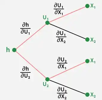
​\frac{dy}{dx} = \frac{df}{dg} \cdot \frac{dg}{dx}

This means that the chain rule enables us to compute:

• The derivative of the loss with respect to output.
• The derivative of output with respect to weights (and biases), layer by layer.

Steps to Implement Chain Rule Derivative

Suppose you have a simple neural network with one input layer (2 features), one hidden layer (2 neurons) and one output layer (1 neuron).
Let’s denote:

• Input: x=[x₁, x₂]
• Weights: W₁ (input to hidden), W₂ (hidden to output)
• Biases: b1 (hidden), b2 (output)
• Activation: \sigma (sigmoid function)
• Output: z (scalar prediction)

Step 1: Forward Pass (Function Composition)

In the forward pass, input data is transformed through each layer using weights, biases and activation functions to produce the network output.

a_1 = \sigma({W}_1 {x} + {b}_1)
z = \sigma({W}_2 a_1 + b_2)

Here, a₁ is the hidden layer’s activation and z is the final output.

Step 2: Loss Function

Here, we compute the loss, which measures the difference between the network predicted output and the true target, using Mean Squared Error (MSE) for training.

L=\frac{1}{2}(z−y)^2

where y is the true target.

Step 3: Chain Rule for Gradients(Backpropagation)

1. Output Layer gradient:

\frac{\partial L}{\partial z} = z - y

2. Gradient of output w.r.t. parameters:

\frac{\partial z}{\partial {W}_2} = z(1 - z){a}_1^T

\frac{\partial z}{\partial b_2} = z(1 - z)

3. Chain Rule applied to Output Layer parameters:

\frac{\partial L}{\partial {W}_2} = \frac{\partial L}{\partial z} \cdot \frac{\partial z}{\partial {W}_2}

\frac{\partial L}{\partial b_2} = \frac{\partial L}{\partial z} \cdot \frac{\partial z}{\partial b_2}

Step 4: Parameter Update

Once we have all gradients, update each parameter with gradient descent (or any modern optimizer):

{W}_1 = {W}_1 - \alpha \frac{\partial L}{\partial{W}_1}

\mathbf{b}_1 = \mathbf{b}_1 - \alpha \frac{\partial L}{\partial \mathbf{b}_1}

{W}_2 = {W}_2 - \alpha \frac{\partial L}{\partial{W}_2}

b_2 = b_2 - \alpha \frac{\partial L}{\partial b_2}

Step-by-Step Implementation

Let's see an example using PyTorch,

Step 1: Import Libraries

Let's import the required libraries,

• Torch: Modern libraries utilize automatic differentiation and GPU acceleration. PyTorch syntax is widely used in research and industry.

import torch
import torch.nn as nn

Step 2: Define the Neural Network Architecture

We prepare a two-layer neural network (input -> hidden -> output) with sigmoid activation.

class SimpleNet(nn.Module):
    def __init__(self):
        super(SimpleNet, self).__init__()
        self.hidden = nn.Linear(2, 2)
        self.output = nn.Linear(2, 1)
        self.sigmoid = nn.Sigmoid()

    def forward(self, x):
        a1 = self.sigmoid(self.hidden(x))
        a2 = self.sigmoid(self.output(a1))
        return a2

Step 3: Set Up Input, Weights and Biases

Weights and biases are automatically initialized.

net = SimpleNet()
x = torch.tensor([[0.5, 1.5]], dtype=torch.float32)

Step 4: Forward Pass: Compute Output

The forward pass computes network output for given input by passing data through layers and activations.

output = net(x)
print(f"Neural Network Output: {output.item():.6f}")

Output:

Neural Network Output: 0.331014

Step 5: Compute Loss and Apply Chain Rule.

Modern frameworks use autograd for derivatives. Let's use MSE loss for simplicity.

target = torch.tensor([[1.0]], dtype=torch.float32)

criterion = nn.MSELoss()
loss = criterion(output, target)
print(f"Loss: {loss.item():.6f}")

loss.backward()

Output:

Loss: 0.447543

Step 6: Access Computed Gradients (Backpropagation)

After calling loss.backward(), gradients are stored and can be accessed for optimization:

print("Gradient for hidden weights:\n", net.hidden.weight.grad)
print("Gradient for output weights:\n", net.output.weight.grad)

Output:

Gradient for hidden weights:
tensor([[0.0023, 0.0068],
[0.0106, 0.0317]])

Gradient for output weights:
tensor([[-0.1109, -0.1770]])

Application

The chain rule plays a crucial role in training and optimizing machine learning models. Key applications include:

• Backpropagation: Updates neural network weights by propagating the loss gradient backward through each layer using the chain rule.
• Gradient Descent Optimization: Computes gradients of the loss with respect to model parameters to iteratively minimize the loss.
• Automatic Differentiation: ML frameworks like TensorFlow and PyTorch use the chain rule to efficiently compute derivatives of complex functions.
• Recurrent Neural Networks (RNNs): Propagates gradients through time steps, enabling learning from sequential data.
• Convolutional Neural Networks (CNNs): Calculates gradients for convolutional layers, allowing the network to learn spatial feature hierarchies.

Advantages

• Automatic Gradient Computation: Enables fast, scalable calculation of gradients, which is essential for training deep neural networks and automating optimization in modern frameworks.
• Practical Backpropagation: Makes efficient backpropagation possible, allowing gradients to be passed through every layer for effective parameter updates.
• Supported by Frameworks: Fully integrated into deep learning libraries like PyTorch, TensorFlow and JAX, which handle chain rule differentiation automatically.
• Architecture Flexibility: Works seamlessly with a wide variety of architectures, including CNNs, RNNs and transformers, supporting diverse machine learning tasks.

Limitations

• Vanishing/Exploding Gradients: Repeated application can lead to gradients becoming too small or too large, causing instability during training.
• Differentiability Requirement: Only applies to functions that are smooth and differentiable; cannot directly handle discrete or non-differentiable operations.
• Computational Cost: For very deep or wide networks, the process can become computationally intensive and memory-heavy.