Logistic Regression is a binary classification algorithm that uses a sigmoid function to model probabilities and offers simplicity, efficiency and interpretability. In this article we will use Logistic Regression to predict diabetes by learning patterns from clinical features and estimating the likelihood of disease occurrence.
Step-by-Step Implementation
Step 1: Import Required Libraries
- Import pandas and numpy are used for data handling and numerical operations
- import seaborn and matplotlib are used for data visualisation
import pandas as pd
import numpy as np
import seaborn as sns
import matplotlib.pyplot as plt
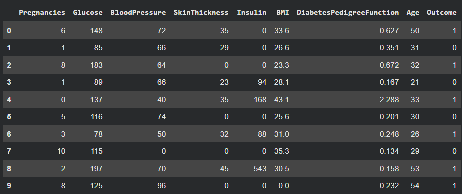
Step 2: Load the Dataset
- The dataset is loaded from a CSV file using pandas
- head() is used to preview the first few records
You can download dataset from here
df = pd.read_csv("diabetes_dataset.csv")
df.head(10)
Output:
Step 3: Data Inspection and Statistical Summary
- isna() checks for missing values in each column
- describe() provides statistical information like mean and standard deviation
df.isna().sum()
df.describe()
Output:
Step 4: Feature and Target Separation
- Independent variables are stored in X
- Dependent variable (Outcome) is stored in y
- Separating features and labels is required for ML models
- This prepares data for training and testing
X = df.drop(columns=['Outcome'])
y = df['Outcome']
Step 5: Train-Test Split
- Data is split into training and testing sets
- 70% data is used for training and 30% for testing
- random_state ensures reproducibility
- This helps evaluate model performance on unseen data
from sklearn.model_selection import train_test_split

X_train, X_test, y_train, y_test = train_test_split(
    X, y, test_size=0.3, random_state=11
)
Step 6: Feature Scaling
- Standardization is applied using StandardScaler
- Scaling improves model convergence and performance
- Logistic Regression performs better with scaled data
- Training and testing data are scaled consistently
from sklearn.preprocessing import StandardScaler

scaler = StandardScaler()
X_train_scaled = scaler.fit_transform(X_train)
X_test_scaled = scaler.transform(X_test)
Step 7: Logistic Regression Model Training
- Logistic Regression is used for binary classification
- max_iter is increased to ensure proper convergence
- The model is trained using scaled training data
from sklearn.linear_model import LogisticRegression

model = LogisticRegression(max_iter=2000)
model.fit(X_train_scaled, y_train)
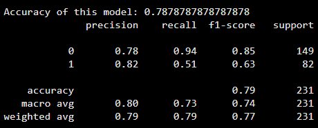
Step 9: Model Prediction and Evaluation
- Predictions are stored in y_pred
- Accuracy score measures overall correctness
- Classification report shows precision, recall, and F1-score
- Confusion matrix provides detailed classification results
from sklearn.metrics import accuracy_score, classification_report, confusion_matrix
y_pred = model.predict(X_test_scaled)
print("Accuracy of this model:", accuracy_score(y_test, y_pred))
print(classification_report(y_test, y_pred))
Output:
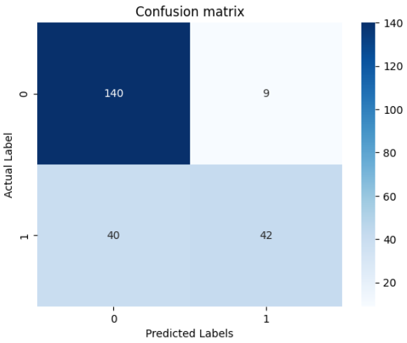
Step 10: Confusion Matrix Visualization
- Confusion matrix is visualized using a heatmap
- It shows true positives, true negatives, false positives, and false negatives
cm = confusion_matrix(y_test, y_pred)

sns.heatmap(cm, annot=True, fmt='d', cmap='Blues')
plt.title("Confusion Matrix")
plt.xlabel("Predicted Labels")
plt.ylabel("Actual Labels")
plt.show()
Output:
You can download full code from here