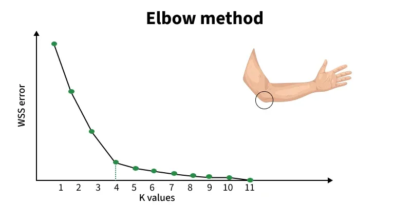
The Elbow Method is used to find the optimal number of clusters (k) in K-Means by analyzing how the clustering performance changes with different k values.
- Plots WCSS (Within-Cluster Sum of Squares) against different k values
- WCSS decreases as k increases, showing better fit
- The “elbow point” indicates the optimal k where improvement slows down
Working of Elbow Point
The Elbow Method works in the following steps:
1. We begin by selecting a range of k values (for example, 1 to 10).
2. For each k, we run K-Means and calculate WCSS (Within-Cluster Sum of Squares), which shows how close the data points are to their cluster centroids:
\text{WCSS} = \sum_{i=1}^{k} \sum_{j=1}^{n_i} \text{distance}(x_j^{(i)}, c_i)^2
Where
3. After computing WCSS for all k values, we plot k vs WCSS.
4. WCSS always decreases as k increases because more clusters reduce the internal spread.
5. However, after a certain point, the improvement becomes very small. This bend or “elbow” in the curve indicates the point where adding more clusters no longer gives meaningful improvement.
- Before the elbow: WCSS drops quickly -> clusters become much better.
- After the elbow: WCSS drops slowly -> extra clusters add little value and may lead to overfitting.
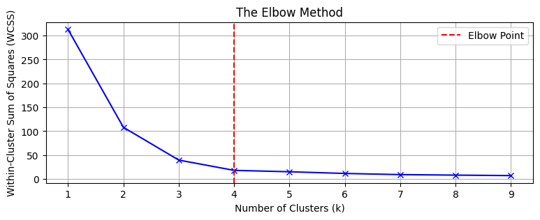
The goal is to identify the point where the rate of decrease in WCSS sharply changes, indicating that adding more clusters (beyond this point) yields diminishing returns. This "elbow" point suggests the optimal number of clusters.
Understanding Distortion and Inertia in K-Means Clustering
Two metrics commonly used in the Elbow Method are Distortion and Inertia.
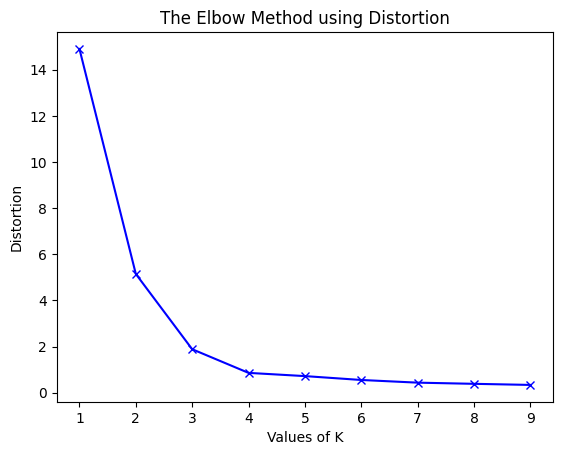
1. Distortion
Distortion measures the average squared distance between each data point and its assigned cluster center. It's a measure of how well the clusters represent the data. A lower distortion value indicates better clustering.
\text{Distortion} = \frac{1}{n} \sum_{i=1}^{n} \min_{c \in \text{clusters}} \left\| x_i - c \right\|^2
where,
x_i is thei^{th} data pointc is a cluster center from the set of all cluster centroids\left\| x_i - c \right\|^2 is the squared Euclidean distance between the data point and the cluster centern is the total number of data points
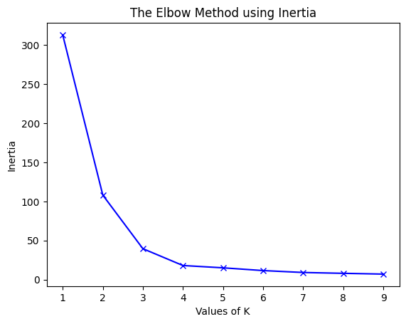
2. Inertia
Inertia is the sum of squared distances of each data point to its closest cluster center. It's essentially the total squared error of the clustering. Like distortion, a lower inertia value suggests better clustering.
\text{Inertia} = \sum_{i=1}^{n} \text{distance}(x_i, c_j^*)^2
In the Elbow Method, we compute distortion or inertia for different k values and plot them. The point where the decrease begins to slow the “elbow” usually indicates the optimal number of clusters.
Implementation of Elbow Method
Let's implement the Elbow method,
Step 1: Importing the required libraries
We will import numpy, matplotlib, scikit learn and scipy for this.
from sklearn.cluster import KMeans
from sklearn import metrics
from scipy.spatial.distance import cdist
import numpy as np
import matplotlib.pyplot as plt
Step 2: Creating and Visualizing the data
We will create a random array and visualize its distribution
x1 = np.array([3, 1, 1, 2, 1, 6, 6, 6, 5, 6,
               7, 8, 9, 8, 9, 9, 8, 4, 4, 5, 4])
x2 = np.array([5, 4, 5, 6, 5, 8, 6, 7, 6, 7,
               1, 2, 1, 2, 3, 2, 3, 9, 10, 9, 10])
X = np.array(list(zip(x1, x2))).reshape(len(x1), 2)

plt.scatter(x1, x2, marker='o')
plt.xlim([0, 10])
plt.ylim([0, 10])
plt.title('Dataset Visualization')
plt.xlabel('Feature 1')
plt.ylabel('Feature 2')
plt.show()
Output:
.png)
From the above visualization, we can see that the optimal number of clusters should be around 3. But visualizing the data alone cannot always give the right answer. Hence we demonstrate the following steps.
Step 3: Building the Clustering Model and Calculating Distortion and Inertia
In this step, we will fit the K-means model for different values of k (number of clusters) and calculate both the distortion and inertia for each value.
distortions = []
inertias = []
mapping1 = {}
mapping2 = {}
K = range(1, 10)

for k in K:
    kmeanModel = KMeans(n_clusters=k, random_state=42).fit(X)

    distortions.append(sum(np.min(cdist(X, kmeanModel.cluster_centers_, 'euclidean'), axis=1)**2) / X.shape[0])

    inertias.append(kmeanModel.inertia_)

    mapping1[k] = distortions[-1]
    mapping2[k] = inertias[-1]
Step 4: Tabulating and Visualizing the Results
a) Displaying Distortion Values
print("Distortion values:")
for key, val in mapping1.items():
    print(f'{key} : {val}')

plt.plot(K, distortions, 'bx-')
plt.xlabel('Number of Clusters (k)')
plt.ylabel('Distortion')
plt.title('The Elbow Method using Distortion')
plt.show()
Output:
Distortion values:
1 : 14.90249433106576
2 : 5.146258503401359
3 : 1.8817838246409675
4 : 0.856122448979592
5 : 0.7166666666666667
6 : 0.5484126984126984
7 : 0.4325396825396825
8 : 0.3817460317460318
9 : 0.3341269841269841
b) Displaying Inertia Values:
print("Inertia values:")
for key, val in mapping2.items():
    print(f'{key} : {val}')

plt.plot(K, inertias, 'bx-')
plt.xlabel('Number of Clusters (k)')
plt.ylabel('Inertia')
plt.title('The Elbow Method using Inertia')
plt.show()
Output:
Inertia values:
1 : 312.95238095238096
2 : 108.07142857142854
3 : 39.51746031746032
4 : 17.978571428571428
5 : 15.049999999999997
6 : 11.516666666666666
7 : 9.083333333333334
8 : 8.016666666666667
9 : 7.0166666666666675
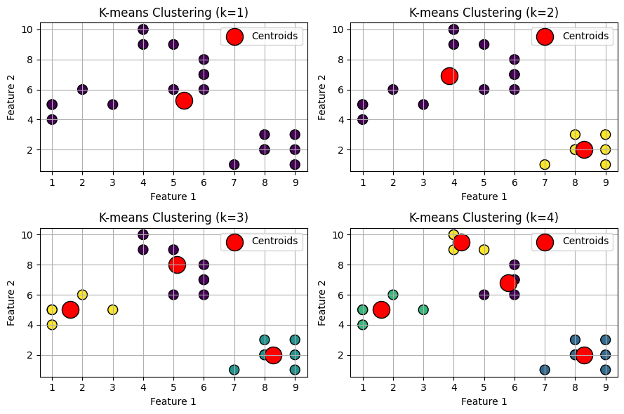
Step 5: Clustered Data Points For Different k Values
We will plot images of data points clustered for different values of k. For this, we will apply the k-means algorithm on the dataset by iterating on a range of k values.
k_range = range(1, 5)

for k in k_range:
    kmeans = KMeans(n_clusters=k, init='k-means++', random_state=42)
    y_kmeans = kmeans.fit_predict(X)

    plt.scatter(X[:, 0], X[:, 1], c=y_kmeans, cmap='viridis', marker='o', edgecolor='k', s=100)
    plt.scatter(kmeans.cluster_centers_[:, 0], kmeans.cluster_centers_[:, 1],
                s=300, c='red', label='Centroids', edgecolor='k')
    plt.title(f'K-means Clustering (k={k})')
    plt.xlabel('Feature 1')
    plt.ylabel('Feature 2')
    plt.legend()
    plt.grid()
    plt.show()
Output:
You can download the source code from here: Source Code