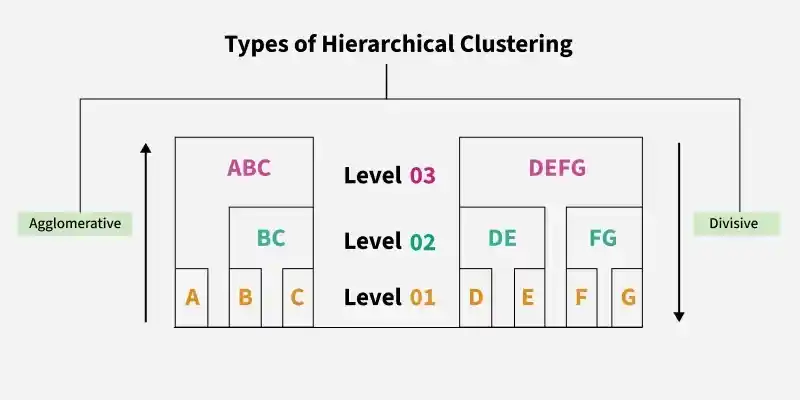
Hierarchical Clustering is an unsupervised learning technique that groups data into a hierarchy of clusters based on similarity. It builds a tree-like structure called a dendrogram, which helps visualise relationships and decide the optimal number of clusters.
- Does not require pre-selecting the number of clusters
- Uses agglomerative (bottom up) or divisive (top down) approaches
- Commonly applied in data exploration and pattern discovery
- Widely used in pattern recognition, customer segmentation and image grouping
Implementing Agglomerative Hierarchical Clustering
Scikit Learn provides a straightforward implementation of Agglomerative hierarchical clustering through the Agglomerative Clustering class.
Step 1: Import Required Libraries
Here we will import numpy, pandas, matplotlib and scikit learn for its implementation.
import numpy as np
import pandas as pd
import matplotlib.pyplot as plt

from sklearn.datasets import load_digits
from sklearn.preprocessing import StandardScaler
from sklearn.cluster import AgglomerativeClustering
from sklearn.metrics import silhouette_score
from scipy.cluster.hierarchy import dendrogram, linkage
Step 2: Load the Dataset
- Each row represents an image flattened into numerical features.
- No labels are used during clustering this is purely unsupervised.
digits = load_digits()
X = digits.data
Step 3: Feature Scaling
Feature scaling matters in Hierarchical Clustering because the algorithm relies on distance calculations and is highly sensitive to feature magnitudes.
scaler = StandardScaler()
X_scaled = scaler.fit_transform(X)
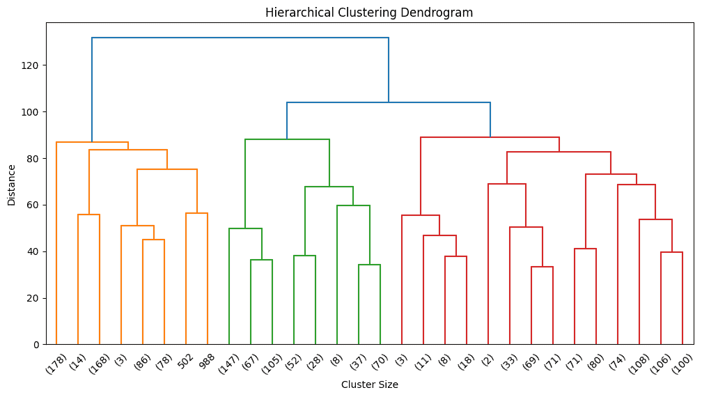
Step 4: Visualizing the Dendrogram
Before selecting the number of clusters, we visualize the hierarchy using a dendrogram.
linked = linkage(X_scaled, method='ward')

plt.figure(figsize=(12, 6))
dendrogram(
    linked,
    truncate_mode='lastp',
    p=30
)
plt.title("Hierarchical Clustering Dendrogram")
plt.xlabel("Cluster Size")
plt.ylabel("Distance")
plt.show()
Output:
Step 5: Building the Hierarchical Clustering Model
Based on dendrogram inspection, we choose a reasonable number of clusters.
hc_model = AgglomerativeClustering(
    n_clusters=10,
    linkage='ward'
)
Step 6: Fit the Model and Assign Clusters
This step fits the hierarchical clustering model to the scaled data and assigns a cluster label to each data point. Each label represents the cluster formed from the hierarchical structure defined by the dendrogram.
cluster_labels = hc_model.fit_predict(X_scaled)
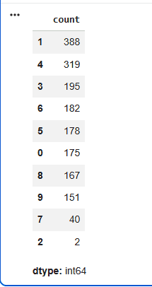
Step 7: Cluster Distribution Analysis
This step shows how data points are distributed across clusters. It provides quick insight into cluster balance, helps detect over fragmentation and highlights dominant groupings, making it an important checkpoint before using the clusters downstream.
pd.Series(cluster_labels).value_counts()
Output:
Step 8: Evaluating Clustering Quality
- The Silhouette Score evaluates how well clusters are formed by comparing cohesion within clusters to separation between clusters.
- Scores closer to +1 indicate well defined clusters, while values near 0 or negative suggest overlap or poor grouping.
sil_score = silhouette_score(X_scaled, cluster_labels)
print("Score :", round(sil_score, 2))
Output:
Score : 0.13
Implementing Divisive Hierarchical Clustering
Scikit Learn does not provide a dedicated library or built in API for divisive clustering. Instead, the approach is implemented manually by applying a top down recursive splitting strategy, most commonly using K Means clustering from scikit learn to divide clusters step by step.
Step 1: Import Required Libraries
Here we will import numpy and scikit learn library.
from sklearn.datasets import load_digits
from sklearn.preprocessing import StandardScaler
from sklearn.cluster import KMeans
from sklearn.metrics import silhouette_score
import numpy as np
Step 2: Load the Dataset
- Each row represents an image flattened into numerical features.
- No labels are used during clustering, this is purely unsupervised.
digits = load_digits()
X = digits.data
Step 3: Feature Scaling
Feature scaling ensures stable and meaningful partitioning.
scaler = StandardScaler()
X_scaled = scaler.fit_transform(X)
Step 4: Defining Divisive Clustering Function
This function applies a top down divisive clustering strategy, where the dataset is repeatedly split into smaller clusters to reveal finer patterns.
- Starts by treating the entire dataset as one cluster
- Splits the cluster into two using K Means
- Recursively repeats the same process on each sub cluster
- Stops when the maximum depth or minimum cluster size is reached
def divisive_clustering(X, depth=0, max_depth=3, min_size=50):

    if depth == max_depth or len(X) <= min_size:
        return [X]


    kmeans = KMeans(n_clusters=2, random_state=42)
    labels = kmeans.fit_predict(X)

    cluster_1 = X[labels == 0]
    cluster_2 = X[labels == 1]


    return (
        divisive_clustering(cluster_1, depth + 1, max_depth, min_size) +
        divisive_clustering(cluster_2, depth + 1, max_depth, min_size)
    )
Step 5: Execute Divisive Clustering
This step applies divisive clustering to the scaled data using the defined depth and minimum size.
final_clusters = divisive_clustering(
    X_scaled,
    max_depth=3,
    min_size=50
)
Step 6: Analyze Cluster Sizes
This step calculates the number of data points in each final cluster to understand how the data has been split.
cluster_sizes = [len(cluster) for cluster in final_clusters]
cluster_sizes
Output:
[39, 568, 643, 369, 178]
Step 7: Assign Flat Cluster Labels
This step transforms the hierarchical, tree based clustering output into flat cluster labels, which are required by most machine learning pipelines to enable evaluation, visualization and deployment.
labels = np.empty(X_scaled.shape[0], dtype=int)

start = 0
for i, cluster in enumerate(final_clusters):
    size = len(cluster)
    labels[start:start + size] = i
    start += size
Step 8: Evaluate Cluster Quality
- The Silhouette Score evaluates how well clusters are formed by comparing cohesion within clusters to separation between clusters.
- Scores closer to +1 indicate well defined clusters, while values near 0 or negative suggest overlap or poor grouping.
sil_score = silhouette_score(X_scaled, labels)
print("Score :", round(sil_score, 2))
Output:
Score : -0.04
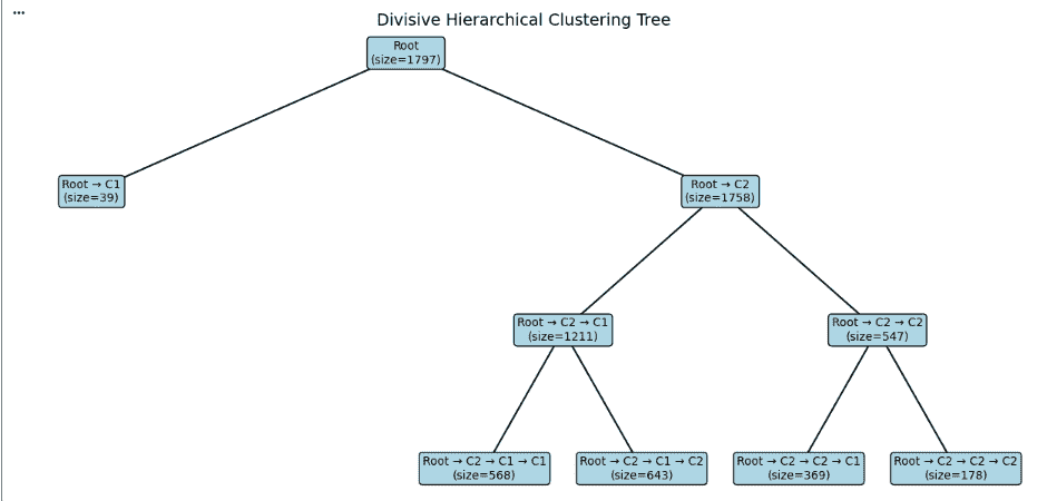
Step 9: Visualizing Divisive Hierarchical Clustering Tree
Now we will visualize the divisive clustering process as a tree.
- Begins with the entire dataset as a single cluster (Root).
- Divides it into two clusters using KMeans.
- Recursively splits each resulting cluster into smaller groups.
- Stops when the maximum depth is reached or the cluster size becomes too small.
def build_tree(X, depth=0, max_depth=3, min_size=50, node_name="Root"):

    if depth == max_depth or len(X) <= min_size:
        return {
            "name": f"{node_name}\n(size={len(X)})",
            "children": []
        }

    kmeans = KMeans(n_clusters=2, random_state=42)
    labels = kmeans.fit_predict(X)

    cluster_1 = X[labels == 0]
    cluster_2 = X[labels == 1]

    return {
        "name": f"{node_name}\n(size={len(X)})",
        "children": [
            build_tree(cluster_1, depth + 1, max_depth, min_size, node_name + " → C1"),
            build_tree(cluster_2, depth + 1, max_depth, min_size, node_name + " → C2")
        ]
    }

tree = build_tree(X_scaled, max_depth=3, min_size=50)
Now, Assigns X and Y positions to each node, where depth controls the vertical placement and child nodes are distributed horizontally to maintain proper spacing.
def compute_positions(node, depth=0, x=0, positions=None, width=8):

    if positions is None:
        positions = {}

    positions[node["name"]] = (x, -depth)

    children = node["children"]
    if children:
        dx = width / len(children)
        start_x = x - width/2 + dx/2

        for i, child in enumerate(children):
            compute_positions(child,
                              depth + 1,
                              start_x + i * dx,
                              positions,
                              width / 2)
    return positions
Now we extract the parent child relationships by recursively traversing the tree. For each node, we store its connection to its children so that these relationships can later be drawn as lines in the visualization. This step builds the structural backbone required to clearly represent the hierarchical clustering tree.
def extract_edges(node, edges=None):

    if edges is None:
        edges = []

    for child in node["children"]:
        edges.append((node["name"], child["name"]))
        extract_edges(child, edges)

    return edges
Now we draw the tree by connecting each parent node to its children and displaying the cluster size inside every node. Colours are used to make the structure easier to read. This creates a clear top down view of how the data was split during divisive clustering.
def plot_tree(tree):

    positions = compute_positions(tree)
    edges = extract_edges(tree)

    fig, ax = plt.subplots(figsize=(12, 6))
    ax.axis('off')


    for parent, child in edges:
        x1, y1 = positions[parent]
        x2, y2 = positions[child]
        ax.plot([x1, x2], [y1, y2], 'k-')


    for node, (x, y) in positions.items():

        if "Root" in node:
            color = "lightblue"
        elif "C1" in node or "C2" in node:
            color = "lightgreen"
        else:
            color = "lightyellow"

        ax.text(x, y, node,
                ha='center',
                va='center',
                bbox=dict(boxstyle="round",
                          facecolor=color,
                          edgecolor="black"))

    plt.title("Divisive Hierarchical Clustering Tree", fontsize=14)
    plt.tight_layout()
    plt.show()
plot_tree(tree)
Output:
You can download the code from here