Hinge loss is a loss function widely used in machine learning for training classifiers such as support vector machines (SVMs). Its purpose is to penalize predictions that are incorrect or insufficiently confident in the context of binary classification. It is used in binary classification problems where the objective is to separate the data points in two classes typically labeled as +1 and -1. Mathematically, Hinge loss for a data point can be represented as :
L(y, f(x)) = max(0, 1 - y * f(x))
Where,
- y the actual class (-1 or 1).
- f(x) the output of the classifier for the datapoint.
Relationship Between Hinge Loss and SVM
In SVMs, the goal is to find a hyperplane that separates classes with the widest possible margin, improving generalization. The model balances maximizing this margin and penalizing misclassified points through the hinge loss. The objective is:
\frac{1}{2} \|w\|^2 + C \sum_{i=1}^n \max\left(0,\, 1 - y_i (w \cdot x_i + b)\right)
where
Step-by-Step Implementation
We will use iris dataset to construct a SVM classifier using Hinge loss.
Step 1: Import Necessary Libraries.
- datasets: Contains standard datasets, like Iris.
- train_test_split: For splitting data into learning (training) and testing parts.
- SGDClassifier: Implements a linear SVM with hinge loss using stochastic gradient descent.
- precision_score, recall_score, confusion_matrix: Evaluation metrics to gauge how well the classifier performs.
from sklearn import datasets
from sklearn.model_selection import train_test_split
from sklearn.linear_model import SGDClassifier
from sklearn.metrics import precision_score, recall_score, confusion_matrix
Step 2: Load the Dataset and Split Data into Training and Test Sets
- load_iris() gives both feature data and target labels for the Iris flowers dataset, a standard for testing classifiers. X refers to the feature matrix (measurements) and y is the set of class labels.
- Divides the dataset into a training set (for fitting the model) and a test set (for evaluating the model’s ability to generalize). Here, 33% is reserved for testing.
iris = datasets.load_iris()
X = iris.data
y = iris.target

X_train, X_test, y_train, y_test = train_test_split(
    X, y, test_size=0.33, random_state=42
)
Step 3: Train an SVM Classifier with Hinge Loss, Make Predictions on the Test Set
- SGDClassifier(loss="hinge") configures a linear SVM using the hinge loss function, just like traditional SVMs.
- max_iter=1000 ensures enough learning steps for the optimizer to potentially converge to a good solution.
- .fit(X_train, y_train) actually learns the hyperplane separating the classes, using only the training samples.
- Applies the trained SVM model to the test data to predict labels, simulating how it would classify new, unseen examples.
clf_hinge = SGDClassifier(loss="hinge", max_iter=1000, random_state=42)
clf_hinge.fit(X_train, y_train)

y_test_pred = clf_hinge.predict(X_test)
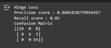
Step 4: Evaluate Model Performance
- Precision: Measures how many predicted positives are truly positive.
- Recall: Shows how many actual positives were correctly predicted.
- Confusion Matrix: Breaks down the types of correct and incorrect predictions across all classes, useful for diagnosing performance in detail.
print("Precision score:", precision_score(
    y_test, y_test_pred, average='weighted'))
print("Recall score:", recall_score(y_test, y_test_pred, average='weighted'))
print("Confusion Matrix:")
print(confusion_matrix(y_test, y_test_pred))
Advantages of using hinge loss for SVMs
There are several advantages to using hinge loss for SVMs:
- Easy to optimize due to its convex nature.
- Pushes SVMs to create the widest possible separation between classes.
- Remains reliable even with some label errors or noise.
- Prioritizes learning from challenging, close-to-margin examples.
Disadvantages
There are a few disadvantages to using hinge loss for SVMs:
- Not differentiable at the margin (zero), which can hinder some optimizers.
- Sensitive to severe outliers.
- Limited to linear and kernel SVMs; not commonly used for all loss-based models.
- Does not provide probability estimates directly.