Predicting house prices is a key challenge in the real estate industry, helping buyers, sellers and investors make informed decisions. By using machine learning algorithms, we can estimate the price of a house based on various features such as location, size, number of bedrooms and other relevant factors.
We will use the House Price Prediction Dataset, which can be downloaded from the provided link. The dataset contains 13 key features:
- Id: Unique identifier for each record.
- MSSubClass: Type of dwelling involved in the sale.
- MSZoning: General zoning classification of the property.
- LotArea: Lot size in square feet.
- LotConfig: Configuration of the lot.
- BldgType: Type of dwelling.
- OverallCond: Overall condition rating of the house.
- YearBuilt: Original construction year.
- YearRemodAdd: Remodel year (same as construction year if no remodeling).
- Exterior1st: Exterior covering of the house.
- BsmtFinSF2: Type 2 finished square feet of the basement.
- TotalBsmtSF: Total basement area in square feet.
- SalePrice: The target variable we aim to predict.
Step 1: Importing Libraries and Dataset
In the first step we load the libraries which is needed for Prediction:
- Import Pandas to load the Dataframe
- Import Matplotlib to visualize the data features
- Import Seaborn to see the correlation between features using heatmap
You can download full dataset from here
import pandas as pd
import matplotlib.pyplot as plt
import seaborn as sns

dataset = pd.read_excel("HousePricePrediction.xlsx")

print(dataset.head(5))
Output:

As we have imported the data. So shape method will show us the dimension of the dataset.
dataset.shape
Output:
(2919,13)
Step 2: Data Preprocessing
Here we categorize the features based on their data types (integer, float, or object) and count the number of features in each category.
object_cols = dataset.select_dtypes(include=['object']).columns
print("Categorical variables:", len(categorical_cols))

int_ = dataset.select_dtypes(include=['int64']).columns
print("Integer variables:", len(integer_cols))

fl_cols = dataset.select_dtypes(include=['float64']).columns
print("Float variables:", len(float_cols))
Output:
Categorical variables: 4
Integer variables: 6
Float variables: 3
Step 3: Exploratory Data Analysis
Exploratory Data Analysis involves examining the dataset in depth to uncover patterns, detect anomalies and understand the underlying structure. Before drawing any conclusions, it’s important to analyze all variables carefully.
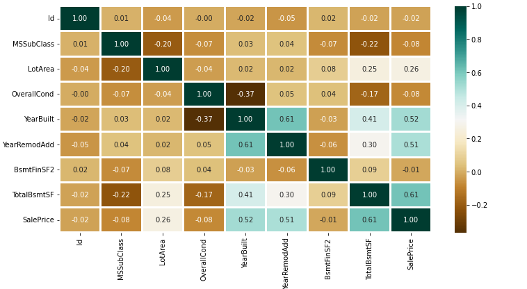
Here we will create a heatmap using the Seaborn library to visualize correlations between features.
numerical_dataset = dataset.select_dtypes(include=['int64', 'float64'])

plt.figure(figsize=(12, 6))
sns.heatmap(numerical_dataset.corr(),
            cmap='BrBG',
            fmt='.2f',
            linewidths=2,
            annot=True)
plt.title("Correlation Heatmap of Numerical Features")
plt.tight_layout()
plt.savefig("correlation_heatmap.png")
print("Heatmap saved as correlation_heatmap.png")
Output:
To examine the categorical features, we will create a bar plot to visualize their distributions
unique_values = []
for col in object_cols:
  unique_values.append(dataset[col].unique().size)
plt.figure(figsize=(10,6))
plt.title('No. Unique values of Categorical Features')
plt.xticks(rotation=90)
sns.barplot(x=object_cols,y=unique_values)
Output:
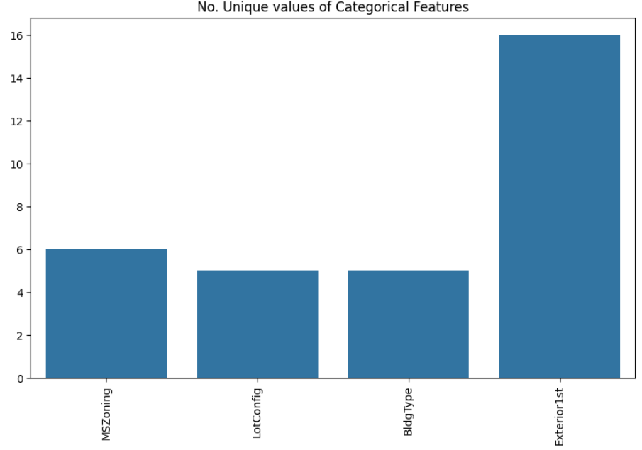
The plot shows that Exterior1st has around 16 unique categories and other features have around 6 unique categories. To findout the actual count of each category we can plot the bargraph of each four features separately.
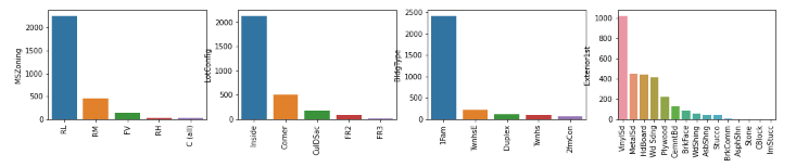
plt.figure(figsize=(18, 36))
plt.title('Categorical Features: Distribution')
plt.xticks(rotation=90)
index = 1

for col in object_cols:
    y = dataset[col].value_counts()
    plt.subplot(11, 4, index)
    plt.xticks(rotation=90)
    sns.barplot(x=list(y.index), y=y)
    index += 1
Output:
Step 4: Data Cleaning
Data Cleaning is the way to improvise the data or remove incorrect, corrupted or irrelevant data. As in our dataset there are some columns that are not important and irrelevant for the model training. So we can drop that column before training. There are 2 approaches to dealing with empty/null values
- We can easily delete the column/row (if the feature or record is not much important).
- Filling the empty slots with mean/mode/0/NA/etc. (depending on the dataset requirement).
As Id Column will not be participating in any prediction. So we can Drop it.
dataset.drop(['Id'],
             axis=1,
             inplace=True)
Replacing SalePrice empty values with their mean values to make the data distribution symmetric.
dataset['SalePrice'] = dataset['SalePrice'].fillna(
  dataset['SalePrice'].mean())
Drop records with null values (as the empty records are very less).
new_dataset = dataset.dropna()
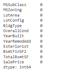
Checking features which have null values in the new dataframe (if there are still any).
new_dataset.isnull().sum()
Output:
Step 5: OneHotEncoder - For Label categorical features
One hot Encoding is the best way to convert categorical data into binary vectors. This maps the values to integer values. By using OneHotEncoder, we can easily convert object data into int. So for that firstly we have to collect all the features which have the object datatype. To do so, we will make a loop.
from sklearn.preprocessing import OneHotEncoder
s = (new_dataset.dtypes == 'object')
object_cols = list(s[s].index)
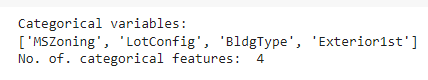
print("Categorical variables:")
print(object_cols)
print('No. of. categorical features: ',
len(object_cols))
Output:
Then once we have a list of all the features. We can apply OneHotEncoding to the whole list.
OH_encoder = OneHotEncoder(sparse_output=False, handle_unknown='ignore')
OH_cols = pd.DataFrame(OH_encoder.fit_transform(new_dataset[object_cols]))
OH_cols.index = new_dataset.index
OH_cols.columns = OH_encoder.get_feature_names_out()
df_final = new_dataset.drop(object_cols, axis=1)
df_final = pd.concat([df_final, OH_cols], axis=1)
Step 6: Splitting Dataset into Training and Testing
X and Y splitting (i.e. Y is the SalePrice column and the rest of the other columns are X)
from sklearn.metrics import mean_absolute_error
from sklearn.model_selection import train_test_split

X = df_final.drop(['SalePrice'], axis=1)
Y = df_final['SalePrice']

X_train, X_valid, Y_train, Y_valid = train_test_split(
    X, Y, train_size=0.8, test_size=0.2, random_state=0)
Step 7: Model Training and Accuracy
As we have to train the model to determine the continuous values, so we will be using these regression models.
- SVM-Support Vector Machine
- Random Forest Regressor
- Linear Regressor
And To calculate loss we will be using the mean_absolute_percentage_error module. It can easily be imported by using sklearn library. The formula for Mean Absolute Error is:
\text{MAE} = \frac{1}{n} \sum_{i=1}^{n} \left| y_i - \hat{y}_i \right|
1. SVM - Support vector Machine
Support vector Machine is a supervised machine learning algorithm primarily used for classification tasks though it can also be used for regression. It works by finding the hyperplane that best divides a dataset into classes. The goal is to maximize the margin between the data points and the hyperplane.
from sklearn import svm
from sklearn.svm import SVC
from sklearn.metrics import mean_absolute_percentage_error

model_SVR = svm.SVR()
model_SVR.fit(X_train,Y_train)
Y_pred = model_SVR.predict(X_valid)

print(mean_absolute_percentage_error(Y_valid, Y_pred))
Output :
0.1870512931870423
2. Random Forest Regression
Random Forest is an ensemble learning algorithm used for both classification and regression tasks. It constructs multiple decision trees during training where each tree in the forest is built on a random subset of the data and features, ensuring diversity in the model. The final output is determined by averaging the outputs of individual trees (for regression) or by majority voting (for classification).
from sklearn.ensemble import RandomForestRegressor

model_RFR = RandomForestRegressor(n_estimators=10)
model_RFR.fit(X_train, Y_train)
Y_pred = model_RFR.predict(X_valid)

mean_absolute_percentage_error(Y_valid, Y_pred)
Output :
0.18602695581046166
3. Linear Regression
Linear Regression is a statistical method used for modeling the relationship between a dependent variable and one or more independent variables. The goal is to find the line that best fits the data. This is done by minimizing the sum of the squared differences between the observed and predicted values. Linear regression assumes that the relationship between variables is linear.
from sklearn.linear_model import LinearRegression

model_LR = LinearRegression()
model_LR.fit(X_train, Y_train)
Y_pred = model_LR.predict(X_valid)

print(mean_absolute_percentage_error(Y_valid, Y_pred))
Output :
0.1874168384159986
Clearly SVM model is giving better accuracy as the mean absolute error is the least among all the other regressor models i.e. 0.18 approx. To get much better results ensemble learning techniques like Bagging and Boosting can also be used.
You can download full code from here