How KNN Imputer Works in Machine Learning

The KNN Imputer is a machine learning–based method for filling missing values in datasets. Instead of using a single statistic (like mean or median), it estimates missing values using the values of the k most similar data points (neighbors).

• Multivariate approach: Considers multiple features simultaneously.
• Data-driven: Uses patterns in the dataset, not external assumptions.
• Robust: Better preserves relationships between variables compared to univariate methods.

Working of K-Nearest Neighbors Imputer

The method is built on the K-Nearest Neighbors (KNN) algorithm, commonly used for classification and regression. The steps are:

• Distance Calculation: Compute distances between the data point with missing values and all others. By default, a NaN-aware Euclidean distance is used.
• Identify Neighbors: Select the k closest neighbors based on computed distances.
• Imputation: Replace the missing value with the average (for continuous data) or majority vote (for categorical data) of the neighbors’ values.
• Multivariate Handling: Takes all available features into account for improved accuracy.

Example: Imputing Missing Values with KNN Imputer

Suppose we have the following dataset,

We will impute the missing values.

Step 1: Identify the Missing Values

Missing value: X_1 in observation 3.

Step 2: Compute Distance

We compute distances between Observation 3 and other observations using features X_2 and X_3 .

Euclidean Distance Formula:

d(a, b) = \sqrt{\sum_{i=1}^{n} (a_i - b_i)^2}

1. Distance between Observation 3 and 1:

d(3,1) = \sqrt{(1.5 - 1.0)^2 + (5.0 - 3.0)^2} = \sqrt{0.25 + 4.0} = \sqrt{4.25} \approx 2.06

2. Distance between Observation 3 and 2:

d(3,2) = \sqrt{(1.5 - 2.0)^2 + (5.0 - 4.0)^2} = \sqrt{0.25 + 1.0} = \sqrt{1.25} \approx 1.12

3. Distance between Observation 3 and 4:

d(3,4) = \sqrt{(1.5 - 3.5)^2 + (5.0 - 6.0)^2} = \sqrt{4.0 + 1.0} = \sqrt{5.0} \approx 2.24

Step 3: Find the Nearest Neighbors

Closest neighbor: Observation 2(1.12) and Observation 1(2.06)

Step 4: Impute the Missing Value

Take the mean of neighbors’ values in X₁:

\text{Imputed Value} = \frac{3.0 \;(\text{Obs 2}) + 2.0 \;(\text{Obs 1})}{2} = \frac{3.0 + 2.0}{2} = 2.5

So, the missing value in X₁ (Observation 3) is imputed as 2.5.

Code Example

Let's see the implementation of using KNN Imputer.

• Import libraries: such as NumPy, Pandas and KNNImputer
• Create dataset: Some values set as np.nan to simulate missing data.
• Convert to DataFrame: Makes the dataset easy to handle.
• Initialize imputer: KNNImputer(n_neighbors=2) uses 2 nearest neighbors for filling missing values.
• Fit and transform: Finds nearest rows and replaces NaN with the average of their values.
• Convert back to DataFrame: Keeps original column names.

import numpy as np
import pandas as pd
from sklearn.impute import KNNImputer

data = {
    'X1': [2.0, 3.0, np.nan, 5.0, 4.0],
    'X2': [1.0, 2.0, 1.5, 3.5, np.nan],
    'X3': [3.0, 4.0, 5.0, 6.0, 4.5]
}

df = pd.DataFrame(data)

imputer = KNNImputer(n_neighbors=2)

imputed_df = pd.DataFrame(imputer.fit_transform(df), columns=df.columns)

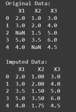
print("Original Data:")
print(df)
print("\nImputed Data:")
print(imputed_df)

Output:

Applications

• Healthcare Data: Filling missing lab test results or patient vitals for more accurate diagnosis models.
• Finance & Banking: Imputing missing transaction or credit history values for risk assessment.
• Retail & E-commerce: Completing missing customer purchase behavior data for recommendation systems.
• Sensor Data / IoT: Handling missing readings in environmental or industrial sensors.
• Survey & Social Science Research: Filling in incomplete responses to maintain dataset usability.

Advantages

• Multivariate approach: Considers correlations between features.
• Flexibility: Works with different distance metrics and values of k.
• Preserves distribution: Maintains dataset integrity better than mean/median filling.

Challenges

• High computation cost: Distance calculation for large datasets is slow.
• Choice of k: Small k may overfit, large k may oversmooth important details.
• Memory usage: Requires storing the full dataset to compute neighbors.
• Not ideal for categorical data: Needs encoding or special handling.