Gradient Boosting Regression is a machine learning technique that builds models sequentially, where each new model corrects the errors of the previous ones. By combining multiple weak learners (like decision trees) it produces a strong predictive model capable of capturing complex patterns in data.
- Builds models step‑by‑step to reduce prediction errors
- Combines many weak decision trees into a strong model
- Widely used for accurate regression tasks in real‑world datasets
1. Importing the Required Libraries
We need to import the necessary libraries such as numpy, pandas, matplotlib and scikit learn.
import numpy as np
import matplotlib.pyplot as plt
import pandas as pd
from sklearn.tree import DecisionTreeRegressor
2. Creating the Dataset
We will generate a random dataset with 100 points, where X is a single feature and y is our target variable.
np.random.seed(42)
X = np.random.rand(100, 1) - 0.5
y = 3 * X[:, 0]**2 + 0.05 * np.random.randn(100)

df = pd.DataFrame()
df['X'] = X.reshape(100)
df['y'] = y

plt.scatter(df['X'], df['y'])
plt.title('X vs Y')
plt.show()
Output:

The scatter plot shows a nonlinear relationship, which we'll use to train our models.
3. Initial Prediction with Mean Value (Model m1)
The first model (m1) is a simple baseline model that predicts the mean of the target values for all inputs. This is our initial prediction. The predicted line will be just a horizontal line at the mean of the target values which is not a good fit for our data.
df['pred1'] = df['y'].mean()
4. Calculating Pseudo-Residuals
Pseudo-residuals are the differences between the actual values and the predictions from the first model. These residuals are what the next model (m2) will try to predict.
df['res1'] = df['y'] - df['pred1']

plt.scatter(df['X'], df['y'])
plt.plot(df['X'], df['pred1'], color='red')
plt.title('Initial Prediction')
plt.show()
Output:

The red line represents the mean value, which poorly fits the nonlinear data, hence the high residuals.
5. Building the Second Model (m2)
The second model (m2) is a decision tree regressor that predicts the pseudo-residuals from the first model. This tree will help us correct the mistakes made by m1.
tree1 = DecisionTreeRegressor(max_leaf_nodes=8)
tree1.fit(df['X'].values.reshape(100, 1), df['res1'].values)
After fitting the tree, we can visualize it:
from sklearn.tree import plot_tree
plot_tree(tree1)
plt.show()
Output:

The decision tree predicts the pseudo-residuals, which helps in adjusting the initial predictions towards the true values.
6. Updating Predictions (Model m2)
We combine the predictions from m1 and m2 to get updated predictions.
X_test = np.linspace(-0.5, 0.5, 500)
y_pred = df['pred1'].iloc[0] + tree1.predict(X_test.reshape(500, 1))

plt.figure(figsize=(14, 4))
plt.plot(X_test, y_pred, linewidth=2, color='red')
plt.scatter(df['X'], df['y'])
plt.title('Updated Prediction with m2')
plt.show()
Output:

This new line fits the data much better than the initial mean value, but we can still improve it.
7. Adding a Third Model (m3)
We can further improve the fit by adding a third model (m3). First, we calculate new pseudo-residuals (res2) and then fit another decision tree (tree2).
df['pred2'] = df['pred1'].iloc[0] + tree1.predict(df['X'].values.reshape(100, 1))
df['res2'] = df['y'] - df['pred2']

tree2 = DecisionTreeRegressor(max_leaf_nodes=8)
tree2.fit(df['X'].values.reshape(100, 1), df['res2'].values)
8. Combining All Models
Now, we combine all predictions (m1, m2, m3) to get the final prediction:
y_pred = df['pred1'].iloc[0] + tree1.predict(X_test.reshape(500, 1)) + tree2.predict(X_test.reshape(500, 1))

plt.figure(figsize=(14, 4))
plt.plot(X_test, y_pred, linewidth=2, color='red')
plt.scatter(df['X'], df['y'])
plt.title('Final Prediction with m3')
plt.show()
Output:
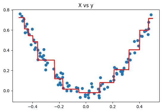
The resulting curve now fits the data even better compared to all 3 models individually. It shows how gradient boosting can be useful to improve models accuracy.
Download the code file from here.