Implementing L1 and L2 regularization using Sklearn

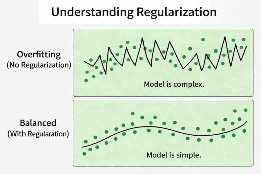
Regularization is a technique used to prevent overfitting in machine learning models. It works by adding a penalty to the loss function so the model does not become too complex. The two most common types are L1 (Lasso) and L2 (Ridge) regularization. Now let us understand the concept in a simple flow:

• We first control model complexity so it does not overfit the training data.
• We then apply L1 regularization, which can reduce some feature coefficients to zero.
• Next, we apply L2 regularization, which reduces coefficient values but keeps all features.
• Finally, we choose the appropriate method depending on whether we want feature selection (L1) or coefficient shrinkage (L2).

Implementation using Scikit Learn

Step 1: Import Required Libraries

• Ridge : L2 Regularization
• Lasso : L1 Regularization

import numpy as np
import pandas as pd
from sklearn.datasets import load_diabetes
from sklearn.model_selection import train_test_split
from sklearn.linear_model import LinearRegression, Ridge, Lasso
from sklearn.metrics import mean_squared_error, r2_score

Step 2: Load the Dataset

• load_diabetes loads a built in regression dataset.
• X contains input features.
• y contains the target values.

data = load_diabetes()
X = data.data
y = data.target

Step 3: Split the Dataset

• 80% of data is used for training and 20% for testing.
• random_state=42 ensures reproducible results.

X_train, X_test, y_train, y_test = train_test_split(
    X, y, test_size=0.2, random_state=42
)

Step 4: Building model without Regularization

• No penalty term is applied
• Model may overfit if data is complex
• This serves as our baseline model

linear_model = LinearRegression()
linear_model.fit(X_train, y_train)

linear_pred = linear_model.predict(X_test)

linear_mse = mean_squared_error(y_test, linear_pred)
linear_r2 = r2_score(y_test, linear_pred)

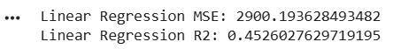
print("Linear Regression MSE:", linear_mse)
print("Linear Regression R2:", linear_r2)

Output:

Step 5: Building model with L1 Regularization

• alpha=0.7 controls penalty strength for L1.
• mean_squared_error() calculates average squared prediction error.
• r2_score() shows how well the model explains variation in the target variable.

lasso_model = Lasso(alpha=0.7)
lasso_model.fit(X_train, y_train)

lasso_pred = lasso_model.predict(X_test)

lasso_mse = mean_squared_error(y_test, lasso_pred)
lasso_r2 = r2_score(y_test, lasso_pred)

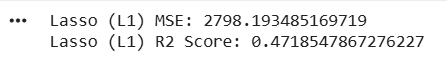
print("Lasso (L1) MSE:", lasso_mse)
print("Lasso (L1) R2 Score:", lasso_r2)

Output:

Step 6: Building model with L2 Regularization

• alpha=1.0 controls regularization strength. Higher alpha means stronger penalty.
• mean_squared_error() calculates average squared prediction error.
• r2_score() shows how well the model explains variation in the target variable.

ridge_model = Ridge(alpha=1.0)
ridge_model.fit(X_train, y_train)

ridge_pred = ridge_model.predict(X_test)

ridge_mse = mean_squared_error(y_test, ridge_pred)
ridge_r2 = r2_score(y_test, ridge_pred)

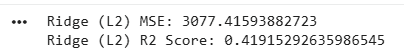
print("Ridge (L2) MSE:", ridge_mse)
print("Ridge (L2) R2 Score:", ridge_r2)

Output:

Download full code from here

Linear Regression vs. L2 vs. L1