K-Nearest Neighbors (KNN) is one of the simplest and most intuitive machine learning algorithms. While it is commonly associated with classification tasks, KNN can also be used for regression.
How KNN Regression Works
- Choosing the number of neighbors (K): The initial step involves selecting the number of neighbors, K. This choice greatly affects the model's performance. A smaller value of K makes the model more prone to noise, whereas a larger value of K results in smoother predictions.
- Calculating distances: For a new data point, calculate the distance between this point and all points in the training set.
- Finding K nearest neighbors: Identify the K points in the training set that are closest to the new data point.
- Predicting the target value: Compute the average of the target values of the K nearest neighbors and use this as the predicted value for the new data point.
Implementing KNN Regression with Scikit-Learn using Synthetic Dataset
Here we demonstrates a practical implementation of KNN regression in Scikit-Learn using a synthetic dataset for illustration.
Step 1: Import Libraries
Here we import NumPy for numerical operations, Matplotlib for visualization and Scikit-learn for data generation, model building and evaluation.
import numpy as np
import matplotlib.pyplot as plt
from sklearn.datasets import make_regression
from sklearn.model_selection import train_test_split
from sklearn.neighbors import KNeighborsRegressor
from sklearn.metrics import mean_squared_error, r2_score
Step 2: Generate Synthetic Dataset
Here we generate a synthetic regression dataset using Scikit-Learn make_regression, specifying the number of samples, a single feature and a small noise level for realism.
X, y = make_regression(n_samples=200, n_features=1, noise=0.1, random_state=42)
Step 3: Split the Dataset
The dataset is split into training and testing sets using train_test_split with 20% of the data reserved for testing to evaluate the model performance on unseen data.
X_train, X_test, y_train, y_test = train_test_split(X, y, test_size=0.2, random_state=42)
Step 4: Create and Train the KNN Regressor
In this step a KNN regressor is created with 5 neighbors and trained on the training dataset to learn the relationship between input features and target values.
knn_regressor = KNeighborsRegressor(n_neighbors=5)
knn_regressor.fit(X_train, y_train)
Output:
Step 5: Make Predictions
The trained KNN regressor generates predictions for the test dataset based on the learned patterns.
y_pred = knn_regressor.predict(X_test)
Step 6: Evaluate the Model
The model performance is evaluated using Mean Squared Error (MSE) to measure prediction error and R-squared to assess how well the model explains the variance in the data.
mse = mean_squared_error(y_test, y_pred)
r2 = r2_score(y_test, y_pred)

print(f'Mean Squared Error: {mse}')
print(f'R-squared: {r2}')
Output:
Mean Squared Error: 133.62045142000457
R-squared: 0.9817384115764595
Step 7: Visualize the Results
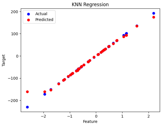
A scatter plot compares the actual versus predicted values, providing a visual assessment of the KNN regression model performance.
plt.scatter(X_test, y_test, color='blue', label='Actual')
plt.scatter(X_test, y_pred, color='red', label='Predicted')
plt.title('KNN Regression')
plt.xlabel('Feature')
plt.ylabel('Target')
plt.legend()
plt.show()
Output:
Implementing KNN Regression with Scikit-Learn using Diabetes Dataset
Here we use the diabetes dataset to perform KNN regression using the following steps:
Step 1: Import Libraries
Import NumPy for numerical operations, Matplotlib for data visualization and Scikit-learn modules for dataset handling, feature scaling, KNN regression and model evaluation.
import numpy as np
import matplotlib.pyplot as plt
from sklearn.datasets import load_diabetes
from sklearn.model_selection import train_test_split
from sklearn.neighbors import KNeighborsRegressor
from sklearn.metrics import mean_squared_error, r2_score
from sklearn.preprocessing import StandardScaler
Step 2: Load the Dataset
The Diabetes dataset is loaded using Scikit-Learn load_diabetes function, providing ten baseline features and a target variable representing disease progression.
diabetes = load_diabetes()
X = diabetes.data
y = diabetes.target

print(diabetes.DESCR)
Step 3: Split the Dataset
The dataset is split into training and testing sets using train_test_split, reserving 20% of the data for evaluating the model performance.
X_train, X_test, y_train, y_test = train_test_split(X, y, test_size=0.2, random_state=42)
Step 4: Standardize the Features
Features are standardized using StandardScaler so that each has a mean of 0 and a standard deviation of 1, improving the performance of the KNN algorithm.
scaler = StandardScaler()
X_train = scaler.fit_transform(X_train)
X_test = scaler.transform(X_test)
Step 5: Create and Train the KNN Regressor
A KNN regressor with 5 neighbors is created and trained on the standardized training data.
knn_regressor = KNeighborsRegressor(n_neighbors=5)
knn_regressor.fit(X_train, y_train)
Step 6: Make Predictions
We use the trained KNN regressor to make predictions on the test data.
y_pred = knn_regressor.predict(X_test)
Step 7: Evaluate the Model
Here, we evaluate the model's performance using the Mean Squared Error (MSE) and R-squared metrics. These metrics help us understand how well the model is performing.
mse = mean_squared_error(y_test, y_pred)
r2 = r2_score(y_test, y_pred)

print(f'Mean Squared Error: {mse}')
print(f'R-squared: {r2}')
Output:
Mean Squared Error: 3047.449887640449
R-squared: 0.42480887066066253
Step 8: Visualize the Results
Finally, we visualize the actual and predicted values using a scatter plot. This step helps us visually assess the model's performance.
plt.figure(figsize=(10, 6))
plt.scatter(y_test, y_pred, color='blue', label='Predicted vs Actual')
plt.plot([min(y_test), max(y_test)], [min(y_test), max(y_test)], color='red', linewidth=2, label='Ideal fit')
plt.title('KNN Regression: Predicted vs Actual')
plt.xlabel('Actual Disease Progression')
plt.ylabel('Predicted Disease Progression')
plt.legend()
plt.show()
Output:

You can download full code from here