Mean Shift clustering is a non-parametric, density-based clustering algorithm that discovers clusters by locating the modes i.e. peaks of the data density in feature space and shifting data points toward those high-density areas until convergence. It does not require specifying the number of clusters in advance it automatically detects the number of clusters and works well for irregularly shaped clusters.
Implementation
Let's see the implementation of mean shift clustering using sklearn:
Step 1: Load the Dataset
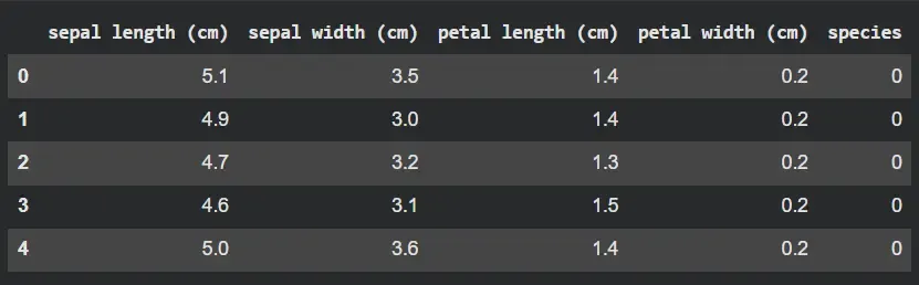
We will import the iris dataset from scikit learn library and print the dataset using pandas.
from sklearn.datasets import load_iris
import pandas as pd

iris = load_iris()
iris_df = pd.DataFrame(iris.data, columns=iris.feature_names)
iris_df["species"] = iris.target
iris_df.head()
Output:
Step 2: Select Features and Scale Them
- X contains all feature columns (sepal length, sepal width, petal length, petal width).
- Mean Shift uses distance-based calculations, so scaling avoids feature dominance.
- StandardScaler standardizes each feature to mean = 0 and variance = 1.
- X_scaled is the normalized data ready for clustering.
from sklearn.preprocessing import StandardScaler
X = iris_df[iris.feature_names].values
scaler = StandardScaler()
X_scaled = scaler.fit_transform(X)
Step 3: Estimate Bandwidth Automatically
- estimate_bandwidth inspects point distances to determine a suitable neighborhood radius.
- quantile=0.2 means bandwidth is based on the 20th percentile of pairwise distances.
- A smaller quantile → smaller bandwidth → more clusters.
- Bandwidth is critical for how Mean Shift behaves, so automatic estimation helps.
- The printed value shows what neighborhood size the algorithm will use.
from sklearn.cluster import estimate_bandwidth
bandwidth = estimate_bandwidth(X_scaled, quantile=0.2, n_samples=len(X_scaled))
print("Estimated Bandwidth:", bandwidth)
Output:
Estimated Bandwidth: 1.207017869625092
Step 4: Apply Mean Shift Clustering
- A MeanShift object is created with the computed bandwidth.
- bin_seeding=True speeds up clustering by using a grid to initialize seeds.
- fit(X_scaled) performs the iterative shifting toward density peaks.
- labels contains the cluster ID assigned to each of the 150 iris samples.
- cluster_centers_ contains the final positions of discovered modes.
- The number of cluster centers indicates how many clusters Mean Shift detected automatically.
from sklearn.cluster import MeanShift
ms = MeanShift(bandwidth=bandwidth, bin_seeding=True)
ms.fit(X_scaled)

labels = ms.labels_
centers_scaled = ms.cluster_centers_
print("Number of clusters found:", len(centers_scaled))
Output:
Number of clusters found: 3
Step 5: Add Cluster Labels to the DataFrame
- A new column cluster is added to store Mean Shift's cluster assignments.
- Printing the first few rows shows how species labels compare to cluster labels.
- crosstab shows the distribution of real species across discovered clusters.
- This helps evaluate how well the unsupervised algorithm separates the species.
iris_df["cluster"] = labels
print(iris_df[["species", "cluster"]].head())
print("\nCluster vs Species:")
print(pd.crosstab(iris_df["cluster"], iris_df["species"]))
Output:

Step 6: Visualize Clusters
Now we will visualize the clusters using matplotlib.
import matplotlib.pyplot as plt
plt.figure(figsize=(7, 5))
plt.scatter(
    iris_df["petal length (cm)"],
    iris_df["petal width (cm)"],
    c=iris_df["cluster"],
    cmap="viridis",
    alpha=0.8
)
plt.xlabel("Petal Length (cm)")
plt.ylabel("Petal Width (cm)")
plt.title("Mean Shift Clustering on Iris Dataset")
plt.colorbar(label="Cluster ID")
plt.show()
Output:
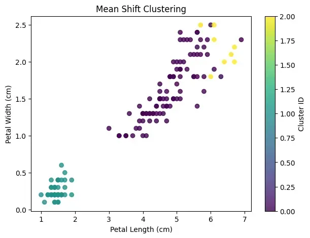
As we can see our model is able to do clustering using Mean Shift Clustering.
Application
- Image segmentation: By grouping pixels into meaningful regions based on color or texture.
- Object tracking: In videos, where Mean Shift follows the highest-density region corresponding to a moving object.
- Dominant color extraction: From images for tasks like palette generation or background isolation.
- Customer segmentation: When the number of customer groups is unknown and clusters may have irregular shapes.
- Geospatial hotspot detection: Such as identifying dense areas of traffic, population or events.