Mean-Shift Clustering

Mean-shift is a density based clustering algorithm that groups data by shifting points toward high density regions. Unlike K-Means, it does not require specifying the number of clusters and can handle complex, irregular cluster shapes.

• Shifts data points iteratively toward the nearest high density region.
• Does not require predefining the number of clusters.
• Works well with clusters of arbitrary shapes and distributions.
• Converges when points reach local maxima, forming final clusters.
• Commonly used in image processing and computer vision.

Mathematical Formulation of Mean-Shift Clustering

Mean-shift is based on estimating the density of data points and moving each point toward the direction of maximum increase in density.

Kernel Density Estimation (KDE)

It is a technique used to estimate the density of data points without assuming any fixed distribution. It works by placing a smooth function around each data point and combining them to form a continuous density surface.

• In Mean-Shift, KDE helps identify high-density regions that act as cluster centres.
• Estimates the probability density of data in a continuous space.
• Does not assume any predefined distribution (non parametric).
• Helps identify high density regions (modes) used for clustering.

The KDE formula is

f(x) = \frac{1}{n h^d} \sum_{i=1}^{n} K\left(\frac{x - x_i}{h}\right)

Where:

• f(x): Estimated density at point x
• n: Total number of data points.
• h: Bandwidth (radius of the kernel), controls smoothness.
• d: Number of dimensions of the data.
• x_i: Each data point in the dataset.
• K: Kernel function that measures influence of nearby points.

Mean Shift Vector

The mean shift vector defines how a data point moves toward regions of higher density. It calculates the direction and distance a point should shift to reach the nearest mode (cluster center).

m(x) = \frac{\sum_{x_i \in N(x)} x_i \, K\left(\frac{x - x_i}{h}\right)}{\sum_{x_i \in N(x)} K\left(\frac{x - x_i}{h}\right)} - x

Where:

• m(x): Mean shift vector, showing direction and magnitude of movement.
• x: Current position of the data point.
• x_i \in N(x): Data points within the neighborhood (radius defined by bandwidth h)
• K\left(\frac{x - x_i}{h}\right): Kernel function that assigns weight based on distance (closer points have higher influence).

Point Update Rule

The point update rule defines how each data point moves during the Mean-Shift process. At every iteration, a point is shifted to the weighted mean of its neighboring points, bringing it closer to a high density region.

x_{\text{new}} = \frac{\sum_{i=1}^{n} x_i \, K\left(\frac{x - x_i}{h}\right)}{\sum_{i=1}^{n} K\left(\frac{x - x_i}{h}\right)}

where:

• x_{\text{new}}: Updated position of the data point after shifting.
• x_i: Neighboring data points in the dataset.
• K\left(\frac{x - x_i}{h}\right): Kernel function that assigns weights based on distance (closer points have higher influence).
• h: Bandwidth (radius) that defines the neighborhood size.

Working of Mean-Shift Clustering

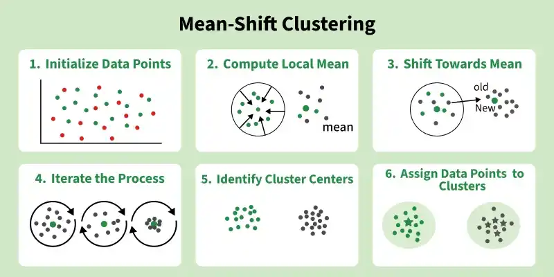
1. Initialize Data Points: All data points are initially treated as potential cluster centroids. Each point will be iteratively updated during the process.
2. Compute Local Mean: For each data point, identify neighboring points within a defined radius (kernel or bandwidth) and calculate their mean position.
3. Shift Towards Mean: Move the data point from its current position to the computed mean, effectively shifting it toward a higher density region.
4. Iterate the Process: Repeat the mean calculation and shifting steps for all points until the movement becomes negligible and points stabilize.
5. Identify Cluster Centers: Points that no longer change position after convergence represent the cluster centers (modes).
6. Assign Data Points to Clusters: Finally, assign each data point to the nearest cluster center, forming the final clusters.

Implementation

Step 1: Import Required Libraries

We will import libraries like pandas, matplotlib and scikit learn.

from sklearn.datasets import load_iris
import pandas as pd
from sklearn.preprocessing import StandardScaler
from sklearn.cluster import estimate_bandwidth
from sklearn.cluster import MeanShift
import matplotlib.pyplot as plt

Step 2: Load Dataset and Create DataFrame

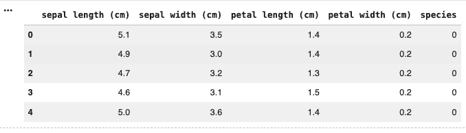
• The Iris dataset is loaded using load_iris() from sklearn.
• A pandas DataFrame is created using feature values like sepal length, petal length, etc.
• A new column species is added to store the actual class labels.

iris = load_iris()

iris_df = pd.DataFrame(iris.data, columns=iris.feature_names)
iris_df["species"] = iris.target
iris_df.head()

Output:

Step 3: Feature Scaling

• Only numerical features are selected for clustering.
• StandardScaler is used to normalize the data so that all features have equal importance.
• Scaling is important because Mean-Shift depends on distance calculations.

X = iris_df[iris.feature_names].values

scaler = StandardScaler()
X_scaled = scaler.fit_transform(X)

Step 4: Estimate Bandwidth

• Bandwidth defines the radius of the neighborhood (kernel size).
• estimate_bandwidth() automatically calculates a suitable value based on the data.
• The quantile parameter controls how tight or loose clusters will be.

from sklearn.cluster import estimate_bandwidth

bandwidth = estimate_bandwidth(X_scaled, quantile=0.2, n_samples=len(X_scaled))
print("Estimated Bandwidth:", bandwidth)

Output:

Estimated Bandwidth: 1.207017869625092

Step 5: Apply Mean-Shift Clustering

• MeanShift model is initialized with the estimated bandwidth.
• fit() trains the model on scaled data.
• labels_ gives the cluster assigned to each data point.
• cluster_centers_ gives the final cluster centers.

ms = MeanShift(bandwidth=bandwidth, bin_seeding=True)
ms.fit(X_scaled)

labels = ms.labels_
centers_scaled = ms.cluster_centers_

print("Number of clusters found:", len(centers_scaled))

Output:

Number of clusters found: 3

Step 6: Add Cluster Labels to Data

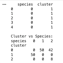
• Cluster labels are added to the DataFrame.
• Comparison between actual species and predicted clusters is shown using a cross tab table.
• This helps evaluate how well clustering matches real categories.

iris_df["cluster"] = labels

print(iris_df[["species", "cluster"]].head())
print("\nCluster vs Species:")
print(pd.crosstab(iris_df["cluster"], iris_df["species"]))

Output:

Step 7: Visualization

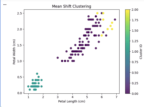
• A scatter plot is created using petal length and width.
• Points are colored based on cluster assignment.
• This visually shows how Mean-Shift has grouped the data.

plt.figure(figsize=(7, 5))

plt.scatter(
    iris_df["petal length (cm)"],
    iris_df["petal width (cm)"],
    c=iris_df["cluster"],
    cmap="viridis",
    alpha=0.8
)

plt.xlabel("Petal Length (cm)")
plt.ylabel("Petal Width (cm)")
plt.title("Mean Shift Clustering")
plt.colorbar(label="Cluster ID")
plt.show()

Output:

Download full code from here

Applications

• Used in image processing for tasks like segmentation and object tracking.
• Applied in computer vision to detect patterns and group similar regions.
• Useful in bioinformatics for clustering gene expression data.
• Can be used in anomaly detection by identifying dense and sparse regions.

Advantages

• Does not require specifying the number of clusters beforehand.
• Can detect clusters of arbitrary shapes and sizes.
• Works well with complex and non linear data distributions.
• Robust to initialization compared to algorithms like K-Means.

Limitations

• Sensitive to the choice of bandwidth, which affects clustering results.
• Computationally expensive for large datasets.
• Performance can degrade with high dimensional data.
• May merge nearby clusters if bandwidth is too large.