Ridge Regressor using sklearn

Ridge Regression is a technique in machine learning that helps prevent overfitting by adding a regularization term to the linear regression model. Using Scikit-Learn, we can implement Ridge Regression to prevent overfitting in linear models.

• Helps prevent overfitting by avoiding fitting noise instead of the actual trend.
• It is a regularised version of linear regression.
• It helps handle highly correlated features by shrinking coefficients, resulting in more stable and accurate predictions.
• Introduces the alpha parameter to control the strength of regularisation.
• Penalises large coefficients to improve model generalisation.

Ridge Regression Loss Function

Ridge Regression aims to minimise both the prediction error and the size of the model coefficients, which is expressed by its cost function:

J(w) = \frac{1}{m} \sum_{i=1}^{m} (\hat{y}_i - y_i)^2 + \frac{\alpha}{2} \sum_{j=1}^{n} w_j^2

where:

• y_{i}: The actual value of the target variable for the i^th data point.
• \hat{y_{i}}: Predicted value of the target variable.
• \alpha: Regularisation parameter that controls the strength of the penalty on large weights.
• J(w): The overall cost (loss) that Ridge Regression tries to minimise.

The first term represents the standard linear regression cost, measuring the mean squared error between predicted and actual values. The second term is the L2 regularization which penalises large coefficients to improve generalisation and prevent overfitting.

How Alpha Controls Regularisation

• If \alpha=0, Ridge Regression reduces to ordinary linear regression.
• A larger \alpha increases regularisation strength, shrinking coefficients toward zero.

Ridge Regression is sensitive to the scale of features, so input features should be standardized.

Choosing the Right \alpha

Selecting an appropriate \alpha is important for balancing bias and variance. Common approaches include:

• Cross-Validation: Test different \alpha values and choose the one with the best performance on unseen data.
• Grid Search: Try a predefined set of \alpha values and select the one that minimizes prediction error.
• Error Metrics: Evaluate using test data rather than training data to avoid overfitting.

Step By Step Implementation

Here we implement Ridge Regression on the California housing dataset.

Step 1: Import Required Libraries

Import essential libraries like

• NumPy for numerical operations
• Matplotlib for visualization
• Scikit learn modules for dataset handling, preprocessing, regression modeling and evaluation

import numpy as np
import matplotlib.pyplot as plt
from sklearn.datasets import fetch_california_housing
from sklearn.model_selection import train_test_split
from sklearn.preprocessing import StandardScaler
from sklearn.linear_model import RidgeCV
from sklearn.metrics import r2_score

Step 2: Load and Split Dataset

Fetch the California housing dataset, assign features (X) and target (y) and split into training and test sets for model training and evaluation.

data = fetch_california_housing()
X = data.data
y = data.target

X_train, X_test, y_train, y_test = train_test_split(X, y, test_size=0.3, random_state=42)

Step 3: Feature Scaling

Standardize the training and test features using StandardScaler to ensure all variables are on the same scale, which improves regression model performance.

scaler = StandardScaler()
X_train_scaled = scaler.fit_transform(X_train)
X_test_scaled = scaler.transform(X_test)

Step 4: Train Ridge Regression with Cross-Validation

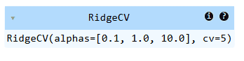
Initialize RidgeCV with multiple alpha values and 5-fold cross-validation, then fit it on the scaled training data to find the optimal regularization strength.

ridge_cv = RidgeCV(alphas=[0.1, 1.0, 10.0], cv=5)
ridge_cv.fit(X_train_scaled, y_train)

Output:

Step 5: Make Predictions and Evaluate Model

Predict housing values on the test set and evaluate model performance using the R² score.

y_pred = ridge_cv.predict(X_test_scaled)

print("Best alpha selected:", ridge_cv.alpha_)
print("Model score (R^2):", r2_score(y_test, y_pred))

Output:

Best alpha selected: 10.0
Model score (R^2): 0.595944060491304

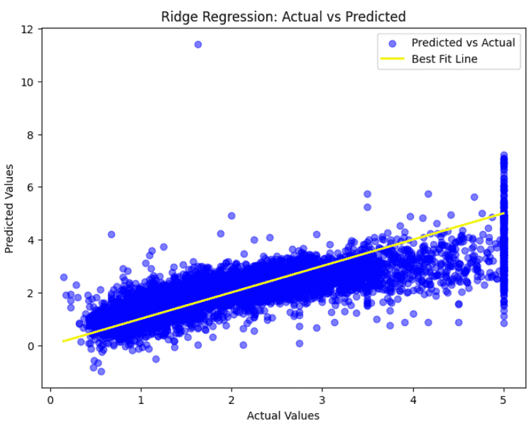
Step 6: Visualize Predictions

Plot the predicted vs actual housing values with a best-fit line to visually assess how well the Ridge Regression model fits the data.

plt.figure(figsize=(8,6))
plt.scatter(y_test, y_pred, color='blue', alpha=0.5, label='Predicted vs Actual')
plt.plot([y_test.min(), y_test.max()], [y_test.min(), y_test.max()], color='yellow', linewidth=2, label='Best Fit Line')
plt.xlabel("Actual Values")
plt.ylabel("Predicted Values")
plt.title("Ridge Regression: Actual vs Predicted")
plt.legend()
plt.show()

Output:

Download code from here.

Limitations

• It retains all features in the model, so it doesn’t help identify which predictors are truly important. This can be confusing in datasets with many features.
• A very high regularization parameter (alpha) can oversimplify the model, causing underfitting and missing important patterns in the data.
• If you expect many coefficients to be exactly zero (sparse solution), Ridge regression is not ideal, unlike Lasso regression which can perform feature selection.
• Although regularization reduces variance, Ridge regression can still be influenced by extreme outliers, which can affect the model’s predictions and coefficients.

Related Articles:

• Ridge Regression in Python
• Ridge Regression in R
• Ridge regression Vs Lasso Regression