ARIMA

ARIMA (Autoregressive Integrated Moving Average) model is used for forecasting time series data. It has some components that allow the model to capture patterns such as trends. For seasonal patterns, an extension called Seasonal ARIMA (SARIMA) is used. Its components are:

1. Autoregression (AR):

The autoregressive part (AR) of an ARIMA model is represented by the parameter p. It signifies the dependence of the current observation on its previous values. Mathematically, an AR(p) model can be represented as:

Y_t=c+\phi_1 Y_{t-1}+\phi_2 Y_{t-2}+\ldots+\phi_p Y_{t-p}+\epsilon_t

Here:

• Y_t is the current observation
• c is a constant
• \phi_1 to \phi_2 are the autoregressive parameters
• \epsilon_t represents the error term at time t

2. Differencing (I):

The differencing part of ARIMA is represented by the parameter d. It involves transforming a non stationary time series into a stationary one by differencing consecutive observations. We can apply the differencing operation multiple times until stationarity is achieved. The formula for differencing is:straightforward

Y_t' = Y_t - Y_{t-1}

Here:

• Y_t' is the differenced series at time t
• Y_t is the original series at time t
• Y_{t-1} is the value of the series at the previous time step

The differencing process is typically applied multiple times until stationarity is achieved. The notation I(d) indicates the order of differencing required for stationarity.

3. Moving Average (MA):

The moving average part (MA) of an ARIMA model is represented by the parameter q. It indicates the dependence of the current observation on the previous forecast errors. Mathematically, an MA(q) model can be represented as:

Y_t=c+\epsilon_t+\theta_1 \epsilon_{t-1}+\theta_2 \epsilon_{t-2}+\ldots+\theta_q \epsilon_{t-q}

Here:

• Y_t is the current observation
• c is a constant
• \epsilon_t is the error at time t
• \theta_1 to \theta_q are the moving average parameters

Working Principles

1. Identifying Stationarity: ARIMA models require the time series data to be stationary. Stationarity implies that the statistical properties of the time series like mean and variance remain constant over time.
2. Parameter Estimation: Estimating the parameters p, d and q involves analyzing the autocorrelation function (ACF) and partial autocorrelation function (PACF) plots of the time series data. ACF helps determine the MA order (q) while PACF aids in determining the AR order (p).
3. Model Fitting: Once the parameters are determined the ARIMA model is fitted to the data. This involves minimizing the error often using methods like maximum likelihood estimation to obtain the most suitable coefficients for the autoregressive and moving average terms.
4. Forecasting: After fitting the model it can be used to forecast future values by iterating over time.

Model Parameters in ARIMA

The ARIMA model is defined by three main parameters: p, d and q.

1. p (AR order): Represents the number of autoregressive terms and is denoted by p. It refers to the number of past observations that directly influence the current value.
2. d (Differencing order): Represents the number of differences needed to make the time series stationary. It involves computing the differences between consecutive observations.
3. q (MA order): Denoted by q it represents the number of lagged forecast errors in the prediction equation.

Selecting the appropriate values for these parameters significantly impacts the model’s forecasting capability. However determining the right values is often a challenging task.

Implementation of ARIMA

We will implement ARIMA model for time series forecasting in Python. This includes steps such as checking for stationarity, performing differencing, analyzing ACF/PACF plots and using grid search to identify the optimal ARIMA parameters for forecasting.

1. Installing Necessary Libraries

We will import the essential Python libraries required for time series analysis.

• pandas, numpy and matplotlib are for data handling and plotting.
• statsmodels provides ARIMA modelling, ADF test (for stationarity) and ACF/PACF plotting tools.
• warnings.filterwarnings('ignore') suppresses warnings to keep the output clean during model fitting and evaluation.

import pandas as pd
import numpy as np
import matplotlib.pyplot as plt
from statsmodels.tsa.arima.model import ARIMA
from statsmodels.tsa.stattools import adfuller
from statsmodels.graphics.tsaplots import plot_acf, plot_pacf
import warnings
import itertools

warnings.filterwarnings('ignore')

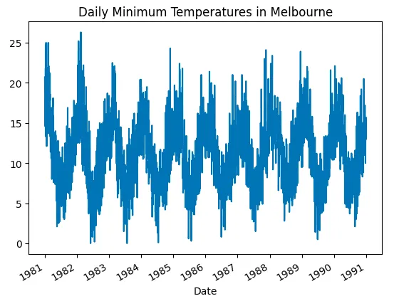
2. Loading the Dataset

We will load the daily temperature dataset from a CSV file, parse the Date column as datetime, and set it as the index.

You can download dataset from here.

• pd.read_csv(): Loads the dataset and parses the Date column as datetime using the parse_dates argument.
• pd.to_numeric(): Converts an argument (typically a series or column) to a numeric type.
• index_col='Date': Sets the Date column as the index for the time series.
• ts.plot(): Plots the time series data to visualize the trend.

data = pd.read_csv('/content/daily-min-temperatures.csv')
data['Temp'] = pd.to_numeric(data['Temp'], errors='coerce')
ts = data['Temp']

ts.plot(title='Daily Minimum Temperatures in Melbourne')
plt.show()

Output:

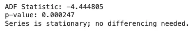
3. Stationarity Check (ADF Test)

We will check if the time series is stationary using the Augmented Dickey-Fuller (ADF) test. We use the adfuller() method to perform the ADF test, which provides the ADF statistic and p-value.

• dropna(): Removes the missing values created after differencing.
• If the p-value is greater than 0.05, the series is non-stationary and differencing is needed.

ts = ts.dropna()
result = adfuller(ts)
print('ADF Statistic: %f' % result[0])
print('p-value: %f' % result[1])

if result[1] > 0.05:
    print("Series is non stationary; differencing is needed.")
else:
    print("Series is stationary; no differencing needed.")

Output:

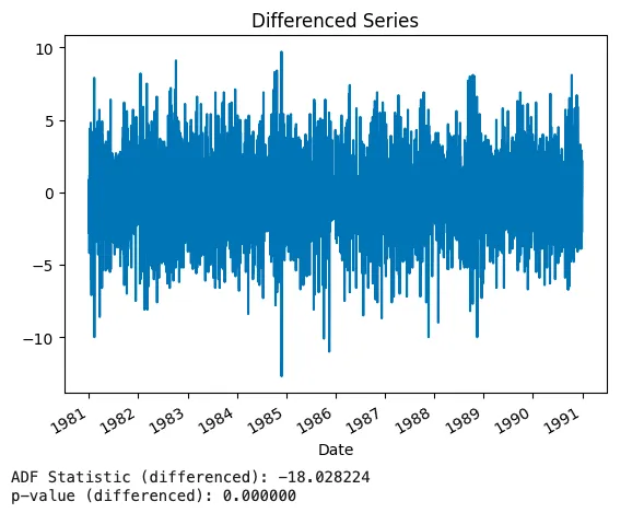
4. Differencing to Achieve Stationarity

We will apply first-order differencing to make the time series stationary if needed and then after differencing, we perform the ADF test again to check if the series is now stationary.

• ts.diff(): Computes the first-order difference of the series to remove trends.
• dropna(): Removes the missing values created after differencing.
• plot(): Visualizes the differenced series.

ts_diff = ts.diff().dropna()

ts_diff.plot(title='Differenced Series')
plt.show()

result_diff = adfuller(ts_diff)
print('ADF Statistic (differenced): %f' % result_diff[0])
print('p-value (differenced): %f' % result_diff[1])

Output:

5. ACF and PACF Plotting (Model Order Identification)

We will plot the ACF and PACF of the differenced series to identify appropriate values for p (AR) and q (MA).

• plot_acf(): Plots the Autocorrelation Function (ACF) to check for the number of MA terms (q).
• plot_pacf(): Plots the Partial Autocorrelation Function (PACF) to check for the number of AR terms (p).

plot_acf(ts_diff)
plt.show()

plot_pacf(ts_diff)
plt.show()

Output:

6. ARIMA Model Selection Using Grid Search

We will perform a grid search over ARIMA (p, d, q) parameters, fit each model and select the best one based on AIC.

• itertools.product(): Generates all combinations of p, d and q for the grid search.
• ARIMA(): Fits the ARIMA model for each combination of p, d and q.
• results.aic: Evaluates the model using the Akaike Information Criterion (AIC), where a lower AIC indicates a better model.

p = range(0, 4)
d = range(0, 3)
q = range(0, 4)
pdq = list(itertools.product(p, d, q))

best_aic = np.inf
best_order = None
best_model = None

for order in pdq:
    try:
        model = ARIMA(ts, order=order)
        results = model.fit()
        if results.aic < best_aic:
            best_aic = results.aic
            best_order = order
            best_model = results
    except:
        continue

print(f'Best ARIMA order: {best_order} with AIC: {best_aic}')

Output:

7. Model Fitting and Forecasting

We will fit the ARIMA model with the best parameters identified earlier and then generate forecasts for future values.

• ARIMA(): Initializes the ARIMA model with the best parameters (p, d, q).
• fit(): Fits the ARIMA model to the time series data and estimates the model's parameters.
• forecast(): Generates forecasts for the specified number of future periods.
• steps: The number of periods into the future for which the forecast is needed.

final_model = ARIMA(ts, order=best_order)
results = final_model.fit()

forecast_values = results.forecast(steps=10)

8: Model Evaluation

We will plot the last 10 values of the original time series data along with the forecasted values to visually assess the model's performance.

• plot(): Plots the original time series data and the forecasted values on the same graph for comparison.
• ts: The original time series data.
• forecast_values: The forecasted values for the future.
• label: Labels to distinguish between the original and forecasted data.

plt.plot(ts[-10:].index, ts[-10:], label='Actual', color='blue', linestyle='-', marker='o')
plt.plot(forecast_values.index, forecast_values, label='Forecast', color='red', linestyle='--', marker='x')

plt.title('ARIMA Forecast: Actual vs Forecast', fontsize=14)
plt.xlabel('Date', fontsize=12)
plt.ylabel('Value', fontsize=12)
plt.legend()
plt.grid(True)
plt.show()

Output:

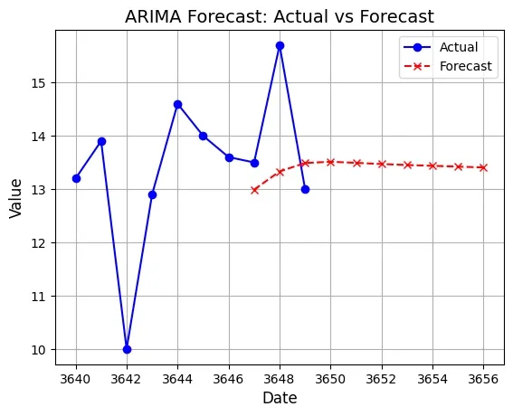
We can improve the model's performance by experimenting with different values of the ARIMA order (p, d, q) or exploring seasonal ARIMA (SARIMA) models if there are seasonal patterns present in the data. Additionally incorporating exogenous variables (ARIMAX) could further enhance the model's predictive accuracy.

You can download source code from here.