SARSA (State-Action-Reward-State-Action) is an on-policy reinforcement learning (RL) algorithm that helps an agent to learn an optimal policy by interacting with its environment. The agent explores its environment, takes actions, receives feedback and continuously updates its behavior to maximize long-term rewards.

Unlike off-policy algorithms like Q-learning which learn from the best possible actions, it updates its knowledge based on the actual actions the agent takes. This makes it suitable for environments where the agent's actions and their immediate feedback directly influence learning.
Components
Components of the SARSA Algorithm are as follows:
- State (S): The current situation or position in the environment.
- Action (A): The decision or move the agent makes in a given state.
- Reward (R): The immediate feedback or outcome the agent receives after taking an action.
- Next State (S'): The state the agent transitions to after taking an action.
- Next Action (A'): The action the agent will take in the next state based on its current policy.
- Discount Factor (γ): Determines how much importance is given to future rewards compared to immediate rewards.
SARSA focuses on updating the agent's Q-values (a measure of the quality of a given state-action pair) based on both the immediate reward and the expected future rewards.
How does SARSA Updates Q-values?
SARSA updates the Q-value using the Bellman Equation for SARSA:
Q(s_t, a_t) \leftarrow Q(s_t, a_t) + \alpha \left[ r_{t+1} + \gamma Q(s_{t+1}, a_{t+1}) - Q(s_t, a_t) \right]
Where:
Q(s_t, a_t) is the current Q-value for the state-action pair at time step t.α is the learning rate (a value between 0 and 1) which determines how much the Q-values are updated.r_{t+1} is immediate reward the agent receives after taking actiona_t in states_t .γ is the discount factor (between 0 and 1) which shows the importance of future rewards.Q(s_{t+1}, a_{t+1}) is the Q-value for the next state-action pair.
Understanding the Update
- Immediate Reward: The agent gets reward
r_{t+1} after taking actiona_t in states_t . - Future Reward: It uses
Q(s_{t+1}, a_{t+1}) to estimate future returns. - Correction: The Q-value is adjusted based on the difference between expected and actual rewards.
This helps the agent improve its decisions step by step.
SARSA Algorithm Steps
Lets see how the SARSA algorithm works step-by-step:
1. Initialize Q-values: Begin by setting arbitrary values for the Q-table (for each state-action pair).
2. Choose Initial State: Start the agent in an initial state
3. Episode Loop: For each episode (a complete run through the environment) we set the initial state
4. Step Loop: For each step in the episode:
- Take action
a_t observe rewardR_{t+1} and transition to the next states_{t+1} . - Choose the next action
a_{t+1} based on the policy for states_{t+1} . - Update the Q-value for the state-action pair
(s_t, a_t) using the SARSA update rule. - Set
s_t = s_{t+1} anda_t = a_{t+1} .
5. End Condition: Repeat until the episode ends either because the agent reaches a terminal state or after a fixed number of steps.
Implementation
Let’s consider a practical example of implementing SARSA in a Grid World environment where the agent can move up, down, left or right to reach a goal.
Step 1: Defining the Environment (GridWorld)
- Start Position: Initial position of the agent.
- Goal Position: Target the agent aims to reach.
- Obstacles: Locations the agent should avoid with negative rewards.
- Rewards: Positive rewards for reaching the goal, negative rewards for hitting obstacles.
GridWorld environment simulates the agent's movement, applying the dynamics of state transitions and rewards.
Here we will be using Numpy library for its implementation.
import numpy as np
import random


class GridWorld:
    def __init__(self, width, height, start, goal, obstacles):
        self.width = width
        self.height = height
        self.start = start
        self.goal = goal
        self.obstacles = obstacles
        self.state = start

    def reset(self):
        self.state = self.start
        return self.state

    def step(self, action):
        x, y = self.state
        if action == 0:
            x = max(x - 1, 0)
        elif action == 1:
            x = min(x + 1, self.height - 1)
        elif action == 2:
            y = max(y - 1, 0)
        elif action == 3:
            y = min(y + 1, self.width - 1)

        next_state = (x, y)

        if next_state in self.obstacles:
            reward = -10
            done = True
        elif next_state == self.goal:
            reward = 10
            done = True
        else:
            reward = -1
            done = False

        self.state = next_state
        return next_state, reward, done
Step 2: Defining the SARSA Algorithm
The agent uses the SARSA algorithm to update its Q-values based on its interactions with the environment, adjusting its behavior over time to reach the goal.
def sarsa(env, episodes, alpha, gamma, epsilon):
    Q = np.zeros((env.height, env.width, 4))

    for episode in range(episodes):
        state = env.reset()
        action = epsilon_greedy_policy(Q, state, epsilon)
        done = False

        while not done:
            next_state, reward, done = env.step(action)
            next_action = epsilon_greedy_policy(Q, next_state, epsilon)

            Q[state[0], state[1], action] += alpha * \
                (reward + gamma * Q[next_state[0], next_state[1],
                 next_action] - Q[state[0], state[1], action])

            state = next_state
            action = next_action

    return Q
Step 3: Defining the Epsilon-Greedy Policy
The epsilon-greedy policy balances exploration and exploitation:
- With probability ϵ, the agent selects a random action (exploration)
- With probability 1 − ϵ, it selects the action with the highest Q-value (exploitation)
To avoid bias when multiple actions have the same Q-value, ties are broken randomly among the best actions.
def epsilon_greedy_policy(Q, state, epsilon):
    if random.uniform(0, 1) < epsilon:
        return random.randint(0, 3)
    else:
        q_values = Q[state[0], state[1]]
        max_q = np.max(q_values)
        best_actions = np.where(q_values == max_q)[0]
        return np.random.choice(best_actions)
Step 4: Setting Up the Environment and Running SARSA
This step involves:
- Defining the grid world parameters like width, height, start, goal, obstacles.
- Setting the SARSA hyperparameters like episodes, learning rate, discount factor, exploration rate.
- Running the SARSA algorithm and printing the learned Q-values.
if __name__ == "__main__":

    width = 5
    height = 5
    start = (0, 0)
    goal = (4, 4)
    obstacles = [(2, 2), (3, 2)]
    env = GridWorld(width, height, start, goal, obstacles)

    episodes = 1000
    alpha = 0.1
    gamma = 0.99
    epsilon = 0.1

    Q = sarsa(env, episodes, alpha, gamma, epsilon)

    print("Learned Q-values:")
    print(Q)
Output:
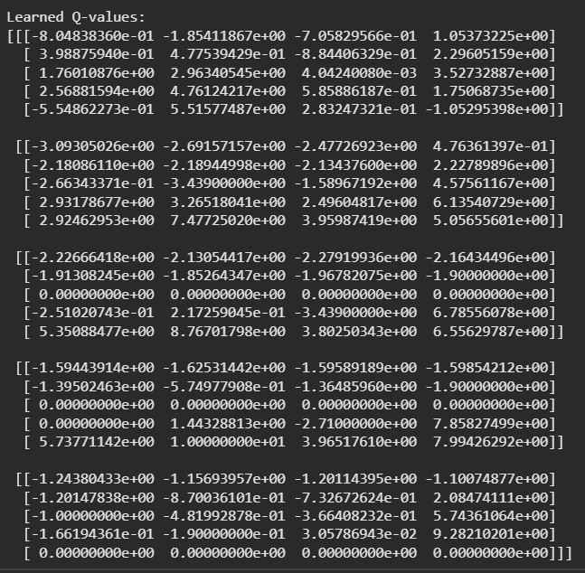
After running the SARSA algorithm the Q-values represent the expected cumulative reward for each state-action pair. The agent uses these Q-values to make decisions in the environment. Higher Q-values shows better actions for a given state.
You can download the complete code from here.
SARSA vs. Q-Learning
| Feature | SARSA (On-Policy) | Q-Learning (Off-Policy) |
|---|---|---|
| Policy Used for Learning | Learns from actions it actually takes | Learns from best possible actions (max Q) |
| Update Uses | Q(s’, a’) | maxaQ(s’, a) |
| Exploration Effect | Included in updates | Ignored in updates |
| Behavior | Learns a safer policy because updates depend on exploration | Learns more aggressive policies |
| Convergence Speed | Slower | Faster |
| Best For | Environments where exploration affects outcomes | Environments where optimal actions are clear |
Exploration Strategies in SARSA
SARSA uses an exploration-exploitation strategy to choose actions. A common strategy is
- Exploration: With probability
ε , the agent chooses a random action (exploring new possibilities). - Exploitation: With probability
1−ε , the agent chooses the action with the highest Q-value for the current state (exploiting its current knowledge).
Over time,
Advantages
- Learns from actual actions taken, making it suitable for environments where exploration directly affects outcomes.
- Produces safer and more realistic behavior since updates consider the agent’s current policy.
- Maintains stability during learning, especially when continuous exploration is required.
- Useful in real-world scenarios where decisions must adapt based on ongoing interaction with the environment.
Limitations
- Converges slower compared to off-policy methods like Q-learning.
- Strongly dependent on the exploration strategy (e.g., ε-greedy), which impacts performance.
- May learn suboptimal policies if exploration is not properly balanced.
- Less efficient in environments where the optimal action is clearly defined.