Self-Supervised Learning (SSL) is a type of machine learning where a model is trained using data that does not have any labels or answers provided. Instead of needing people to label the data, the model finds patterns and creates its own labels from the data automatically.
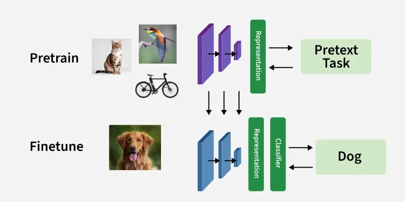
This allows the model to learn useful information by teaching itself from the data. SSL is especially useful when there is a lot of data but only a small part of it is labelled or labelling the data would take a lot of time and effort.
- Uses Unlabeled Data: The model learns directly from raw data without needing humans to label it.
- Dynamic Label Generation: The model generates training labels by understanding the data structure itself.
- Mix of Learning Methods: SSL is a middle ground between supervised learning (with labels) and unsupervised learning (without labels).
- Learns Useful Features: By learning from the data itself, the model can understand important patterns and details which helps it perform better on new data.
- Wide Applications: It is widely used in areas like image recognition, natural language processing and speech recognition, where labeled data can be expensive or limited.
- Helps Transfer Learning: SSL makes it easier to adapt models to new tasks by using the knowledge gained from pre-training on unlabeled data.
Training a Self-Supervised Learning Model in ML
Step 1: Import Libraries and Load Dataset
We will import the required libraries such as TensorFlow, Keras, numpy, matplotlib.pyplot. Also we will load the MNIST dataset for our model.
- Loads MNIST digit images and intentionally ignores the labels for the self-supervised pre-training task.
- Normalizes pixel values to be between 0 and 1.
- Adds a channel dimension to images to fit CNN input shape.
import tensorflow as tf
from tensorflow.keras import layers, models
import numpy as np

(x_train, _), (x_test, _) = tf.keras.datasets.mnist.load_data()

x_train = x_train.astype('float32') / 255.
x_test = x_test.astype('float32') / 255.
x_train = np.expand_dims(x_train, -1)
x_test = np.expand_dims(x_test, -1)

x_train_small = x_train[:1000]
x_test_small = x_test[:200]
Step 2: Prepare Rotation Task Dataset
- Defines four rotation angles (0°, 90°, 180°, 270°) as prediction targets.
- Rotates each image by these angles and records the rotation label.
- Creates a new dataset where the task is to predict the rotation angle, forming a self-supervised task
angles = [0, 90, 180, 270]


def rotate_images(images, angles):
    rotated_images = []
    labels = []
    for img in images:
        for i, angle in enumerate(angles):
            rotated = tf.image.rot90(img, k=angle // 90)
            rotated_images.append(rotated.numpy())
            labels.append(i)
    return np.array(rotated_images), np.array(labels)


x_train_rot, y_train_rot = rotate_images(x_train_small, angles)
x_test_rot, y_test_rot = rotate_images(x_test_small, angles)
Step 3: Define and Compile CNN Model for Rotation Classification
- Defines a simple CNN with convolutional and pooling layers to learn image features.
- The last layer outputs probabilities over 4 classes (rotation angles).
- Compiles the model with Adam optimizer and sparse categorical crossentropy loss for classification.
model = models.Sequential([
    layers.Input(shape=(28, 28, 1)),
    layers.Conv2D(32, 3, activation='relu'),
    layers.MaxPooling2D(),
    layers.Conv2D(64, 3, activation='relu'),
    layers.MaxPooling2D(),
    layers.Flatten(),
    layers.Dense(128, activation='relu'),
    layers.Dense(len(angles), activation='softmax')
])

model.compile(optimizer='adam',
              loss='sparse_categorical_crossentropy',
              metrics=['accuracy'])
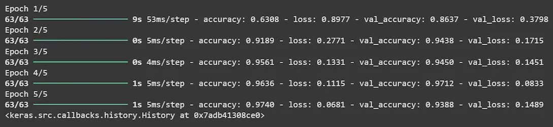
Step 4: Train the Model on Rotated Images
- Trains the model on the self-supervised rotation prediction task.
- Uses the generated rotation labels as targets.
- Validates on a similar rotated test set to monitor performance.
model.fit(x_train_rot, y_train_rot, epochs=5, batch_size=64,
          validation_data=(x_test_rot, y_test_rot))
Output:
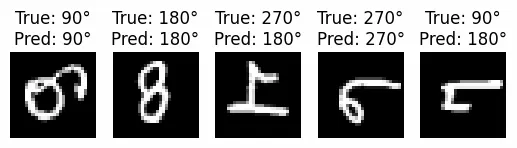
Step 5: Visualized Rotation Predicted Results
- Uses the trained model to predict rotation angles on test images.
- Randomly selects 5 rotated images to display.
- Shows original image with true and predicted rotation angle to check model accuracy visually.
import matplotlib.pyplot as plt

predictions = model.predict(x_test_rot)

num_examples = 5
indices = np.random.choice(len(x_test_rot), num_examples, replace=False)

for i, idx in enumerate(indices):
    img = x_test_rot[idx].squeeze()
    true_label = y_test_rot[idx]
    pred_label = np.argmax(predictions[idx])

    plt.subplot(1, num_examples, i + 1)
    plt.imshow(img, cmap='gray')
    plt.title(f"True: {angles[true_label]}°\nPred: {angles[pred_label]}°")
    plt.axis('off')

plt.show()
Output:
Step 6: Load Labeled MNIST Data for Fine-Tuning
- Loads fully labeled MNIST dataset for downstream digit classification task.
- Preprocesses images and selects smaller subsets for quick fine-tuning.
(x_train_labeled, y_train_labeled), (x_test_labeled,
                                     y_test_labeled) = tf.keras.datasets.mnist.load_data()

x_train_labeled = x_train_labeled.astype('float32') / 255.
x_test_labeled = x_test_labeled.astype('float32') / 255.
x_train_labeled = np.expand_dims(x_train_labeled, -1)
x_test_labeled = np.expand_dims(x_test_labeled, -1)

x_train_fine = x_train_labeled[:1000]
y_train_fine = y_train_labeled[:1000]
x_test_fine = x_test_labeled[:200]
y_test_fine = y_test_labeled[:200]
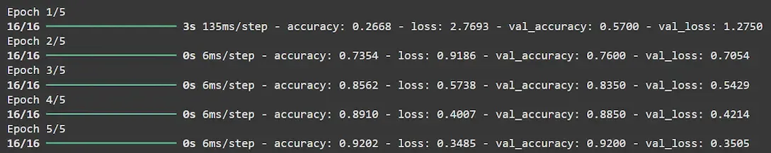
Step 7: Modify and Fine-Tune Model on Labeled Digital Data
- Freezes convolutional layers to keep learned features unchanged.
- Replaces output layer to predict 10 digit classes instead of rotations.
- Compiles and trains the model on labeled data to adapt it for digit recognition.
for layer in model.layers[:-2]:
    layer.trainable = False

model.pop()
model.add(layers.Dense(10, activation='softmax'))

model.compile(optimizer='adam',
              loss='sparse_categorical_crossentropy',
              metrics=['accuracy'])

model.fit(x_train_fine, y_train_fine, epochs=5, batch_size=64,
          validation_data=(x_test_fine, y_test_fine))
Output:
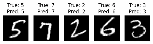
Step 8: Visualize Fine-Tuned Predictions
- Predicts digit classes on labeled test images after fine-tuning.
- Randomly selects 5 test images to display.
- Shows images with ground truth and predicted digit labels for visual performance check.
predictions = model.predict(x_test_fine)

indices = np.random.choice(len(x_test_fine), 5, replace=False)

for i, idx in enumerate(indices):
    img = x_test_fine[idx].squeeze()
    true_label = y_test_fine[idx]
    pred_label = np.argmax(predictions[idx])

    plt.subplot(1, 5, i + 1)
    plt.imshow(img, cmap='gray')
    plt.title(f"True: {true_label}\nPred: {pred_label}")
    plt.axis('off')

plt.show()
Output:
Applications
- Computer Vision: Improves image tasks like recognition, detection, and analysis using unlabeled data.
- NLP: Improves language understanding and tasks like translation and sentiment analysis.
- Speech Recognition: Learns from audio data to transcribe and understand speech.
- Healthcare: Supports diagnosis and analysis where labeled data is limited.
- Autonomous Systems: Helps robots and self-driving systems learn from sensor and video data.
Advantages
- Less Dependence on Labeled Data: Learns useful features from large amounts of unlabeled data, reducing the cost and time of manual labeling.
- Better Generalization: Models learn from the data’s inherent structure, helping them perform well on new, unseen data.
- Supports Transfer Learning: Pre-trained SSL models can be adapted easily to related tasks, speeding up training and improving accuracy.
- Scalable: Can handle very large datasets without the need for expensive annotations, making it ideal for big data scenarios.
Limitations
- Quality of Supervision Signal: The automatically generated labels (pseudo-labels) can be noisy or incomplete, leading to lower accuracy compared to supervised learning.
- Task Restrictions: Less effective for highly complex or unstructured data where meaningful pretext tasks are difficult to design.
- Training Complexity: SSL methods like contrastive learning require careful design, tuning and more computational resources.
- High Computational Cost: Training SSL models often demands significant computation power and time, especially on large datasets.