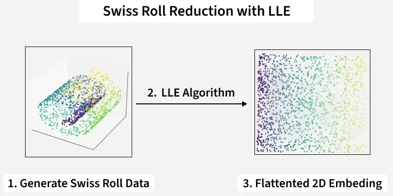
The Swiss roll dataset is a popular non-linear dataset used to test dimensionality reduction algorithms. Even though it appears in 3D, its true structure lies on a 2D surface. Methods like LLE help “unroll” this curved shape and reveal its underlying pattern. It is useful for testing non-linear dimensionality reduction and structure preservation techniques.
Understanding LLE Algorithm
Locally Linear Embedding (LLE) is a manifold learning algorithm used for nonlinear dimensionality reduction. It assumes each data point and its neighbors lie on a locally linear patch of the manifold and preserves these local relationships in a lower-dimensional space. It works by:
- Constructing a neighborhood graph: Each point is connected to its nearest neighbors.
- Finding reconstruction weights: Each point is represented as a linear combination of its neighbors.
- Embedding the data: Lower-dimensional coordinates are computed by minimizing reconstruction error.
LLE can be sensitive to the number of neighbors chosen and may not preserve the global shape of the dataset.
Note: Nonlinear techniques like Locally Linear Embedding (LLE) and t-SNE are better at preserving the curved structure but are more computationally expensive.
Implementation of Swiss Roll Reduction with LLE
We will implement swiss roll reduction using LLE using scikit-learn library.
1. Importing Required Libraries
We begin by importing the Python libraries required for generating data, performing dimensionality reduction and visualization.
- numpy: For numerical operations and handling arrays.
- matplotlib: For plotting 2D graphs and visualizing data.
- mplot3d: Enables 3D plotting for visualizing 3D datasets.
- Sklearn: used to create synthetic 3D data with make_swiss_roll, apply nonlinear dimensionality reduction with LocallyLinearEmbedding and perform linear dimensionality reduction with PCA.
import numpy as np
import matplotlib.pyplot as plt
from mpl_toolkits.mplot3d import Axes3D
from sklearn.datasets import make_swiss_roll
from sklearn.manifold import LocallyLinearEmbedding
from sklearn.decomposition import PCA
2. Generating Swiss Roll Dataset
Next, we create the synthetic 3D dataset that will be used for the experiment.
- make_swiss_roll: Creates a nonlinear 3D manifold (Swiss Roll).
- color array: Maintains consistent colors for visualization.
X, color = make_swiss_roll(n_samples=1000, noise=0.05)
3. Appling Locally Linear Embedding (LLE)
We now perform nonlinear dimensionality reduction using LLE to map the data into 2D.
- n_components=2: Reduces the data to 2D.
- n_neighbors=12: Defines the size of the local neighborhood.
- fit_transform(): Projects data into lower dimensions.
- reconstruction_error_: Measures how well local structure is preserved.
lle = LocallyLinearEmbedding(n_components=2, n_neighbors=12)
X_lle = lle.fit_transform(X)
lle_error = lle.reconstruction_error_
4. Appling Principal Component Analysis (PCA)
For comparison, we also reduce the data using PCA, a linear dimensionality reduction technique.
- PCA: Provides a linear method for dimensionality reduction.
- pca_error: Represents the portion of variance not captured.
pca = PCA(n_components=2)
X_pca = pca.fit_transform(X)
pca_error = 1 - np.sum(pca.explained_variance_ratio_)
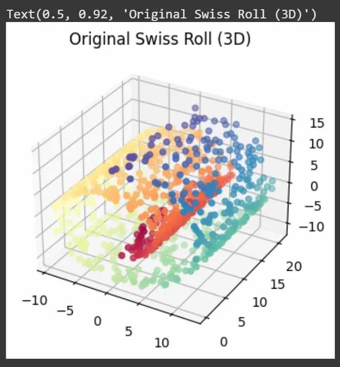
5. Plotting Original Swiss Roll in 3D
We then visualize the original dataset to understand its structure before reduction.
- ax = fig.add_subplot(131, projection='3d'): Adds the first subplot in a 1x3 grid layout and specifies it as a 3D plot.
- ax.scatter(X[:, 0], X[:, 1], X[:, 2], c=color, cmap=plt.cm.Spectral): Plots the 3D data points from the Swiss Roll dataset. The
c=colorargument applies a color mapping based on thecolorarray, whileplt.cm.Spectralprovides a distinct colormap.
fig = plt.figure(figsize=(15, 4))
ax = fig.add_subplot(131, projection='3d')
ax.scatter(X[:, 0], X[:, 1], X[:, 2], c=color, cmap=plt.cm.Spectral)
ax.set_title('Original Swiss Roll (3D)')
Output:
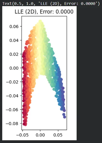
6. Plotting 2D Output from LLE
Here, we visualize the 2D representation obtained from the LLE algorithm.
- Flattening: LLE unrolls the spiral while maintaining neighborhood relationships.
- Manifold learning: Shows effectiveness in capturing nonlinear structure.
plt.subplot(132)
plt.scatter(X_lle[:, 0], X_lle[:, 1], c=color, cmap=plt.cm.Spectral)
plt.title(f'LLE (2D), Error: {lle_error:.4f}')
Output:
7. Plotting 2D Output from PCA
Finally, we display the 2D output from PCA to see how it handles the same dataset.
- Linear projection: PCA projects the data linearly and cannot preserve the spiral structure.
- Color gradient: May still reflect partial ordering despite distortion.
plt.subplot(133)
plt.scatter(X_pca[:, 0], X_pca[:, 1], c=color, cmap=plt.cm.Spectral)
plt.title(f'PCA (2D), Error: {pca_error:.4f}')
Output:
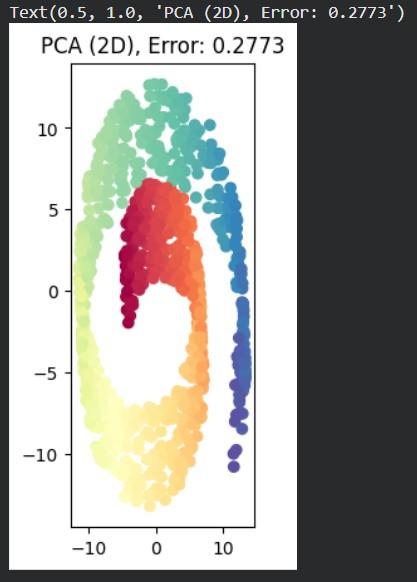
The plots help us compare how well LLE and PCA keep the original shape of the Swiss Roll after reducing it to 2D. The numbers in the plot titles show the error values. LLE and PCA use different error measures, so their values should not be directly compared as each reflects different aspects of dimensionality reduction.
You can download the complete code here.