Understanding Decision Boundaries in K-Nearest Neighbours (KNN)

A decision boundary is a line or surface that divides different groups in a classification task. It shows which areas belong to which class based on what the model decides. K-Nearest Neighbours (KNN) algorithm operates on the principle that similar data points exist in close proximity within a feature space.

The shape of this boundary depends on:

• The value of K (how many neighbours are considered).
• How the data points are spread out in space.

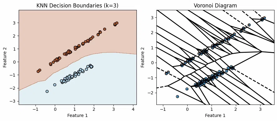
For example, given a dataset with two classes the decision boundary can be visualized as the line or curve dividing the two regions where each class is predicted. For a 1-nearest neighbour (1-NN) classifier the decision boundary can be visualized using a Voronoi diagram.

Using Voronoi Diagrams to Visualize

• A Voronoi diagram splits space into regions based on which training point is closest.
• Each region called a Voronoi cell contains all the points closest to one specific training point.
• The lines between regions are where points are equally close to two or more seeds. These are the decision boundaries for 1-Nearest Neighbour which is very irregular in shape.
• If we label the training points by class the Voronoi diagram shows how KNN assigns a new point based on which region it falls into.
• The boundary line between two points p_i and p_j is the perpendicular bisector of the line joining them meaning it’s a line that cuts the segment between them exactly in half at a right angle.

Relationship between KNN and Voronoi

In two-dimensional space the decision boundaries of KNN can be visualized as Voronoi diagrams. Here’s how:

• KNN Boundaries: The decision boundary for KNN is determined by regions where the classification changes based on the nearest neighbors. As k increases, the decision boundary becomes smoother and less sensitive to local variations, and for very large k, the model may predict the majority class for most regions.
• Voronoi Diagram as a Special Case: When k = 1 KNN’s decision boundaries directly correspond to the Voronoi diagram of the training points. Each region in the Voronoi diagram represents the area where the nearest training point is closest.

How KNN Defines Decision Boundaries

In KNN, decision boundaries are influenced by the choice of k and the distance metric used:

1. Impact of 'K' on Decision Boundaries: The number of neighbors (k) affects the shape and smoothness of the decision boundary.

• Small k: When k is small the decision boundary can become very complex, closely following the training data. This can lead to overfitting.
• Large k: When k is large the decision boundary smooths out and becomes less sensitive to individual data points, potentially leading to underfitting.

2. Distance Metric: The decision boundary is also affected by the distance metric used like Euclidean, Manhattan. Different metrics can lead to different boundary shapes.

• Euclidean Distance: Commonly used leading to circular or elliptical decision boundaries in two-dimensional space.
• Manhattan Distance: Results in axis-aligned decision boundaries.

Decision Boundaries for Different K

Consider a binary classification problem with two features where the goal is to visualize how KNN decision boundary changes as k varies. This example uses synthetic data to illustrate the impact of different k values on the decision boundary.

For a two-dimensional dataset decision boundary can be plotted by:

• Creating a Grid: Generate a grid of points covering the feature space.
• Classifying Grid Points: Use the KNN algorithm to classify each point in the grid based on its neighbors.
• Plotting: Color the grid points according to their class labels and draw the boundaries where the class changes.

import numpy as np
import matplotlib.pyplot as plt
from sklearn.datasets import make_classification
from sklearn.neighbors import KNeighborsClassifier


X, y = make_classification(n_samples=200, n_features=2, n_informative=2, n_redundant=0, n_clusters_per_class=1, random_state=42)

x_min, x_max = X[:, 0].min() - 1, X[:, 0].max() + 1
y_min, y_max = X[:, 1].min() - 1, X[:, 1].max() + 1
xx, yy = np.meshgrid(np.arange(x_min, x_max, 0.01), np.arange(y_min, y_max, 0.01))

fig, axs = plt.subplots(2, 2, figsize=(12, 10))
k_values = [1, 3, 5, 10]

for ax, k in zip(axs.flat, k_values):

    knn = KNeighborsClassifier(n_neighbors=k)
    knn.fit(X, y)
    
    Z = knn.predict(np.c_[xx.ravel(), yy.ravel()])
    Z = Z.reshape(xx.shape)

    ax.contourf(xx, yy, Z, alpha=0.3, cmap=plt.cm.Paired)
    ax.scatter(X[:, 0], X[:, 1], c=y, edgecolor='k',
               cmap=plt.cm.Paired, marker='o')
    ax.set_title(f'KNN Decision Boundaries (k={k})')
    ax.set_xlabel('Feature 1')
    ax.set_ylabel('Feature 2')

plt.tight_layout()
plt.show()

Output:

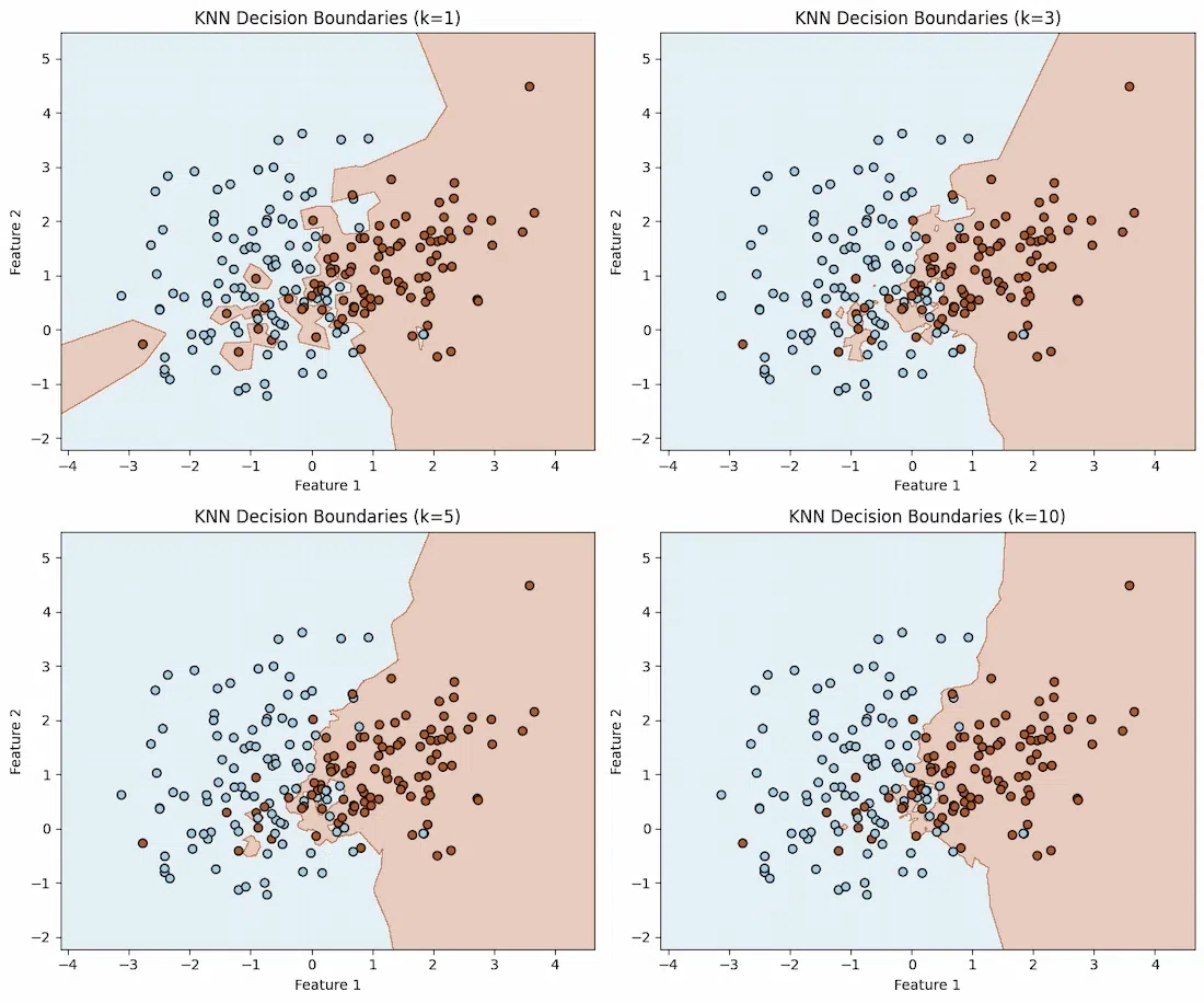
• For small k the boundary is highly sensitive to local variations and can be irregular.
• For larger k the boundary smooths out, reflecting a more generalized view of the data distribution.

Factors affecting KNN Decision Boundaries

• Feature Scaling: KNN is sensitive to the scale of data. Features with larger ranges can dominate distance calculations, affecting the boundary shape.
• Noise in Data: Outliers and noisy data points can shift or distort decision boundaries, leading to incorrect classifications.
• Data Distribution: How data points are spread across the feature space influences how KNN separates classes.
• Boundary Shape: A clear and accurate boundary improves classification accuracy, while a messy or unclear boundary can lead to errors.

Understanding these boundaries helps in optimizing KNN's performance for specific datasets.