Bagging Classifier

Bagging or Bootstrap Aggregating, works by training multiple base models independently and in parallel on different random subsets of the training data. These subsets are created using bootstrap sampling, where data points are randomly selected with replacement, allowing some samples to appear multiple times while others may be excluded.

• In classification tasks, the final prediction is decided by majority voting, the class chosen by most base models.
• For regression tasks, predictions are averaged across all base models, known as bagging regression.
• Bagging is versatile and can be applied with various base learners such as decision trees, support vector machines or neural networks.
• Ensemble learning broadly combines multiple models to create stronger predictive systems by leveraging their collective strengths.

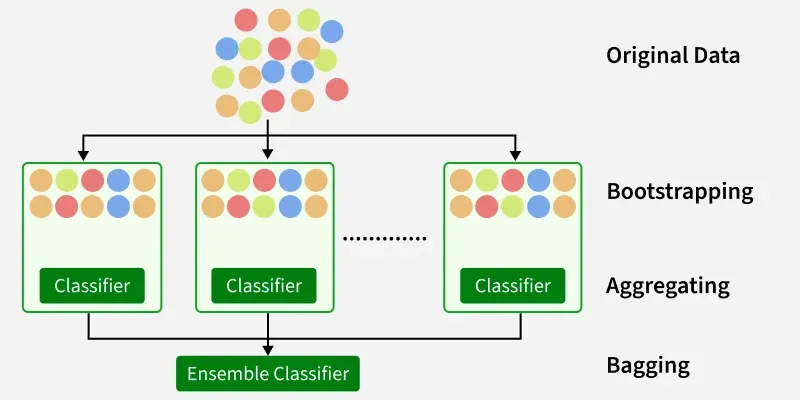
Starting with an original dataset containing multiple data points (represented by colored circles). The original dataset is randomly sampled with replacement multiple times. This means that in each sample, a data point can be selected more than once or not at all. These samples create multiple subsets of the original data.

• For each of the bootstrapped subsets, a separate classifier (e.g., decision tree, logistic regression) is trained.
• The predictions from all the individual classifiers are combined to form a final prediction. This is often done through a majority vote (for classification) or averaging (for regression).

Bagging helps improve accuracy and reduce overfitting especially in models that have high variance.

Working of Bagging Classifier

• Bootstrap Sampling: From the original dataset, multiple training subsets are created by sampling with replacement. This generates diverse data views, reducing overfitting and improving model generalization.

Let's break it down step by step:
Original training dataset: [1, 2, 3, 4, 5, 6, 7, 8, 9, 10]
Resampled training set 1: [2, 3, 3, 5, 6, 1, 8, 10, 9, 1]
Resampled training set 2: [1, 1, 5, 6, 3, 8, 9, 10, 2, 7]
Resampled training set 3: [1, 5, 8, 9, 2, 10, 9, 7, 5, 4]

• Base Model Training: Each bootstrap sample trains an independent base learner (e.g., decision trees, SVMs, neural networks). These “weak learners” may not perform well alone but contribute to ensemble strength. Training happens in parallel, making bagging efficient.
• Aggregation: Once trained, each base model generates predictions on new data. For classification, predictions are combined via majority voting; for regression, predictions are averaged to produce the final outcome.
• Out-of-Bag (OOB) Evaluation: Samples excluded from a particular bootstrap subset (called out-of-bag samples) provide a natural validation set for that base model. OOB evaluation offers an unbiased performance estimate without additional cross-validation.

Bagging starts with the original training dataset.

• From this, bootstrap samples (random subsets with replacement) are created. These samples are used to train multiple weak learners, ensuring diversity.
• Each weak learner independently predicts outcomes, capturing different patterns.
• Predictions are aggregated using majority voting, where the most voted output becomes the final classification.
• Out-of-Bag (OOB) evaluation measures model performance using data not included in each bootstrap sample.
• Overall, this approach improves accuracy and reduces overfitting.

Implementation

Let's see the implementation of Bagging Classifier,

Step 1: Import Libraries

We will import the necessary libraries such as numpy and sklearn for our model,

import numpy as np
from sklearn.tree import DecisionTreeClassifier
from sklearn.datasets import load_digits
from sklearn.model_selection import train_test_split
from sklearn.metrics import accuracy_score

Step 2: Define BaggingClassifier Class and Initialize

• Create the class with base_classifier and n_estimators as inputs.
• Initialize class attributes for the base model, number of estimators and a list to hold trained models.

import numpy as np


class BaggingClassifier:
    def __init__(self, base_classifier, n_estimators):
        self.base_classifier = base_classifier
        self.n_estimators = n_estimators
        self.classifiers = []

Step 3: Implement the fit Method to Train Classifiers

For each estimator:

• Perform bootstrap sampling with replacement from training data.
• Train a fresh instance of the base classifier on sampled data.
• Save the trained classifier in the list.

def fit(self, X, y):
    for _ in range(self.n_estimators):
        indices = np.random.choice(len(X), len(X), replace=True)
        X_sampled, y_sampled = X[indices], y[indices]
        clf = self.base_classifier.__class__()
        clf.fit(X_sampled, y_sampled)
        self.classifiers.append(clf)
    return self.classifiers

Step 4: Implement the predict Method Using Majority Voting

• Collect predictions from each trained classifier.
• Use majority voting across all classifiers to determine final prediction.

def predict(self, X):
    predictions = np.array([clf.predict(X) for clf in self.classifiers])
    majority_votes = np.apply_along_axis(
        lambda x: np.bincount(x).argmax(), axis=0, arr=predictions)
    return majority_votes

Step 5: Load Data

We will,

• Use sklearn's digits dataset.
• Split data into training and testing sets.

digits = load_digits()
X, y = digits.data, digits.target

X_train, X_test, y_train, y_test = train_test_split(
    X, y, test_size=0.2, random_state=42)

Step 6: Train Bagging Classifier and Evaluate Accuracy

• Create a base Decision Tree classifier.
• Train the BaggingClassifier with 10 estimators on training data.
• Predict on test data and compute accuracy.

base_clf = DecisionTreeClassifier()
model = BaggingClassifier(base_classifier=base_clf, n_estimators=10)
model.fit(X_train, y_train)

y_pred = model.predict(X_test)
print("Accuracy:", accuracy_score(y_test, y_pred))

Output:

Accuracy: 0.9166666666666666

Step 7: Evaluate Each Classifier's Individual Performance

• For each trained classifier, predict on test data.
• Print individual accuracy scores to observe variability.

for i, clf in enumerate(model.classifiers):
    y_pred_i = clf.predict(X_test)
    acc_i = accuracy_score(y_test, y_pred_i)
    print(f"Accuracy of classifier {i+1}: {acc_i:.4f}")

Output:

Accuracy of classifier 1: 0.8222
Accuracy of classifier 2: 0.8417
Accuracy of classifier 3: 0.8306
Accuracy of classifier 4: 0.8444
Accuracy of classifier 5: 0.8583
Accuracy of classifier 6: 0.8194
Accuracy of classifier 7: 0.8333
Accuracy of classifier 8: 0.8389
Accuracy of classifier 9: 0.8361
Accuracy of classifier 10: 0.8278

Applications

• Fraud Detection: Enhances detection accuracy by aggregating predictions from multiple fraud detection models trained on different data subsets.
• Spam Filtering: Improves spam email classification by combining multiple models trained on different samples of spam data.
• Credit Scoring: Boosts accuracy and robustness of credit scoring systems by leveraging an ensemble of diverse models.
• Image Classification: Used to increase classification accuracy and reduce overfitting by averaging results from multiple classifiers.
• Natural Language Processing (NLP): Combines predictions from multiple language models to improve text classification and sentiment analysis tasks.

Advantages

• Combines multiple models to reduce overfitting and improve accuracy.
• Reduces the impact of noise and outliers, making results more stable.
• Lowers variance by training on different samples, improving generalization.
• Works with various models like decision trees, SVMs, and neural networks.

Disadvantages

• Does not reduce bias, so errors remain if base models are biased.
• Can still overfit if base models are too complex.
• Offers limited improvement for already stable models.
• Requires proper tuning of parameters for best results.