What is Sparse Categorical Crossentropy

Sparse Categorical Crossentropy is a loss function commonly used in multi-class classification problems in machine learning and deep learning and is particularly used when dealing with a large number of categories. It is very similar to Categorical Crossentropy but with one important difference i.e the true class labels are provided as integers (category indices), not as one-hot encoded vectors.

It is specifically designed for situations where the target labels are provided as integer class indices (e.g., 0, 1, 2, …) rather than one-hot encoded vectors. The term "sparse" refers to this compact label representation which avoids the memory and computational overhead of converting the labels into lengthy one-hot encoded arrays.

Working of Sparse Categorical Crossentropy

• For each input sample, the model predicts a probability distribution over all classes (often using a softmax activation in the final layer).
• The true label for each sample is given as an integer specifying the correct class index.
• Sparse Categorical Crossentropy calculates the negative log-likelihood of the predicted probability assigned to the true class. It only considers the predicted probability associated with the actual class (as marked by the integer label), ignoring all other classes.
• The overall loss is typically the average across all samples in the batch.

The function can be defined as:

L(y, \hat{y}) = -\sum_{i=1}^C y_i \log(\hat{y}_i)

where:

• y is the one-hot encoded true label (a vector),
• \hat y is the predicted probability distribution for all C classes.

Sparse categorical cross entropy modifies this by using the integer index of the true class directly. The loss for each sample is:

L(y, \hat{y}) = -\log\left(\hat{y}_y\right)

where:

• y is the integer index of the correct class,
• \hat y_y  is the predicted probability of the true class output by the model.

Implementation of Sparse Categorical Crossentropy

We will see step by step procedure to implement it in python:

Step 1: Import libraries

Here we will load scikit learn and tensorflow for its implementation.

from sklearn.datasets import load_iris
from sklearn.model_selection import train_test_split
from sklearn.preprocessing import StandardScaler
import tensorflow as tf

Step 2: Load and Preprocess the Data

• load_iris(): Loads flower data with 4 features (like petal length, width, etc.)
• StandardScaler: Normalizes feature values to have mean=0 and std=1.
• train_test_split: 80% data used for training, 20% for testing.

data = load_iris()
X, y = data.data, data.target

X = StandardScaler().fit_transform(X)

X_train, X_test, y_train, y_test = train_test_split(
    X, y, test_size=0.2, random_state=42)

Step 3: Build the Neural Network Model

Make a neural network model which has:

• First layer: 16 neurons, ReLU activation, input shape of 4 (number of features).
• Output layer: 3 neurons (one per flower class).

model = tf.keras.Sequential([
    tf.keras.layers.Dense(16, activation='relu', input_shape=(4,)),
    tf.keras.layers.Dense(3)
])

Step 4: Compile and Train the Model

• Adam optimizer for neural networks.
• Here keras.losses.SparseCategoricalCrossentropy calls Sparse Categorical Crossentropy.
• Trains for 20 epochs on training data.
• Tracks accuracy on validation (test) data too.

model.compile(optimizer='adam',
              loss=tf.keras.losses.SparseCategoricalCrossentropy(
                  from_logits=True),
              metrics=['accuracy'])

model.fit(X_train, y_train, epochs=20, validation_data=(X_test, y_test))

Step 5: Make Predictions

• predict(): Gives raw scores (logits) from the last layer.
• softmax: Converts logits into class probabilities.
• argmax: Picks the class with the highest probability.

import numpy as np

logits = model.predict(X_test)
probs = tf.nn.softmax(logits).numpy()
preds = np.argmax(probs, axis=1)

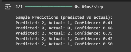
print("\nSample Predictions (predicted vs actual):")
for i in range(5):
    print(
        f"Predicted: {preds[i]}, Actual: {y_test[i]}, Confidence: {np.max(probs[i]):.2f}")

Output:

Application

• Image Classification: Used in tasks like CIFAR-10, MNIST or ImageNet where each image belongs to one class. Labels are integers, making it perfect for sparse crossentropy.
• Text Classification: Applied in spam detection, sentiment analysis or news topic labeling. We assign one label to a full sentence or document using integer-coded classes.
• Product Categorization: In e-commerce, classifying products into thousands of categories is easier and faster with sparse integer labels instead of large one-hot vectors.
• Intent Detection in Chatbots: Classifying user queries into intents like “book flight”, “cancel order” or “track shipment” then here sparse labels make training efficient.
• App Notifications / Alert Systems: Used in classifying alerts or user actions into predefined types hence helping in real-time systems make quick decisions using sparse class targets.

Advantages

• Memory Efficient: We use class labels as integers instead of large one-hot vectors which saves space, especially with many classes.
• Faster Training: No need to convert labels to one-hot encoding which reduces preprocessing time.
• Great for Multi-Class Problems: Ideal for tasks where one sample belongs to exactly one out of many classes like image or text classification.
• Built-In Support in Frameworks: Fully supported in TensorFlow, Keras and PyTorch with optimized backends.

Limitations

• Only for Single-Label Classification: Cannot be used when each input belongs to multiple classes i.e., multi-label problems.
• No Class Probability Control: Less intuitive than one-hot when needing per-class weighting or masking.
• Confusing When Labels Are Preprocessed: We must ensure our labels are integer-encoded (not one-hot) or else we will get errors.
• Harder to Interpret Probabilities: Compared to categorical crossentropy, it’s slightly less transparent when visualizing loss/error distribution across classes.