Bidirectional LSTM in NLP

Bidirectional Long Short-Term Memory (BiLSTM) is an extension of LSTM that processes sequences in both forward and backward directions, allowing the model to capture both past and future context.

• Processes sequences in forward and backward directions
• Captures both past and future contextual information
• More effective than standard LSTMs for sequence understanding
• Commonly used in NLP, speech processing and sequence analysis

Understanding Bidirectional LSTM (BiLSTM)

A Bidirectional LSTM (BiLSTM) consists of two separate LSTM layers:

• Forward LSTM: Processes the sequence from start to end
• Backward LSTM: Processes the sequence from end to start

The outputs of both LSTMs are then combined to form the final output. Mathematically, the final output at time t is computed as:

p_t = p_{t_f} + p_{t_b}

Where:

• p_t: Final probability vector of the network.
• p_{tf}: Probability vector from the forward LSTM network.
• p_{tb}: Probability vector from the backward LSTM network.

The following diagram represents the BiLSTM layer:

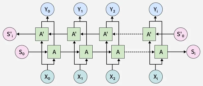
Here:

• X_i is the input token 
• Y_i is the output token
• A and A' are Forward and backward LSTM units
• The final output of Y_i is the combination of A and A' LSTM nodes.

Implementing Sentiment Analysis Using BiLSTM

1. Importing Libraries

We will be using python libraries like numpy, pandas , matplotlib and tensorflow libraries for building our model.

import tensorflow as tf
import tensorflow_datasets as tfds
import numpy as np
import matplotlib.pyplot as plt

2. Loading and Preparing the IMDB Dataset

We will load IMDB dataset from tensorflow which contains 25,000 labeled movie reviews for training and testing. Shuffling ensures that the model does not learn patterns based on the order of reviews.

dataset = tfds.load('imdb_reviews', as_supervised=True)
train_dataset, test_dataset = dataset['train'], dataset['test']

batch_size = 32

train_dataset = train_dataset.shuffle(10000).batch(batch_size)
test_dataset = test_dataset.batch(batch_size)

Printing a sample review and its label from the training set.

example, label = next(iter(train_dataset))
print('Text:\n', example.numpy()[0])
print('\nLabel: ', label.numpy()[0])

Output:

Text: b "Having seen men Behind the Sun ... 1 as a treatment of the subject)."
Label: 0

3. Performing Text Vectorization

We will first perform text vectorization and let the encoder map all the words in the training dataset to a token. We can also see in the example below how we can encode and decode the sample review into a vector of integers.

• vectorize_layer : tokenizes and normalizes the text. It converts words into numeric values for the neural network to process easily.

vectorize_layer = tf.keras.layers.TextVectorization(
    output_mode='int', output_sequence_length=100)

vectorize_layer.adapt(train_dataset.map(lambda x, y: x))

4. Defining Model Architecture (BiLSTM Layers)

The model uses BiLSTM layers for sentiment analysis by processing text sequences in both forward and backward directions.

• TextVectorization converts text into token indices
• Embedding maps words into trainable 32-dimensional vectors
• First Bidirectional(LSTM(32)) captures sequence context and returns sequences
• Dropout(0.4) reduces overfitting
• Second Bidirectional(LSTM(16)) refines learned features
• Another Dropout(0.4) improves generalization
• Dense(16, activation='relu') learns higher-level patterns
• Final dense layer outputs sentiment prediction

model = tf.keras.Sequential([
    vectorize_layer,
    tf.keras.layers.Embedding(
        len(vectorize_layer.get_vocabulary()), 64, mask_zero=True),
    tf.keras.layers.Bidirectional(
        tf.keras.layers.LSTM(64, return_sequences=True)),
    tf.keras.layers.Bidirectional(tf.keras.layers.LSTM(32)),
    tf.keras.layers.Dense(64, activation='relu'),
    tf.keras.layers.Dense(1)
])

model.build(input_shape=(None,))


model.compile(
    loss=tf.keras.losses.BinaryCrossentropy(from_logits=True),
    optimizer=tf.keras.optimizers.Adam(),
    metrics=['accuracy']
)

model.summary()

Output:

5. Training the Model

Now we will train the model we defined in the previous step for three epochs.

history = model.fit(
    train_dataset,
    epochs=3,
    validation_data=test_dataset,
)

Output:

• The model learns well on training data reaching 95.92% accuracy but struggles with validation data staying around 78%.
• The increasing validation loss shows overfitting meaning the model remembers training data but doesn't generalize well.
• To fix this we can use L2 regularization, early stopping or simplify the model to improve real-world performance.

6. Prediction

Lets test our model on sample example to see its working.

review = tf.constant(["This movie was amazing and engaging"])
prob = tf.sigmoid(model.predict(review))[0][0]

sentiment = "Positive" if prob >= 0.5 else "Negative"
print(f"Sentiment: {sentiment}, Probability: {prob:.2f}")

Output:

You can download source code from here.