Moving averages in a Pandas DataFrame are used to smooth time series data and identify overall trends by reducing short-term fluctuations. They help in making patterns more visible and easier to analyze.
In Pandas, we commonly calculate moving averages using:
- Simple Moving Average (SMA): Uses a fixed rolling window to compute the average of recent values.
- Exponential Moving Average (EMA): Gives more weight to recent data, making it more responsive to changes.
- Cumulative Moving Average (CMA): Computes the average from the beginning up to the current point.

Visualizing Stock Trends
Here we create a dataset of stock prices over 15 days and applies different moving average techniques to smooth daily fluctuations and identify trends.
It calculates:
- SMA (Simple Moving Average) using a 5 day rolling window to average recent prices.
- EMA (Exponential Moving Average) which gives more weight to recent values and reacts faster to changes.
- CMA (Cumulative Moving Average) which computes the average from the start up to each day.
import pandas as pd
import numpy as np
import matplotlib.pyplot as plt

data = {'Date': pd.date_range(start='2024-01-01', periods=15, freq='D'),
        'Stock Price': [100, 102, 101, 105, 107, 110, 108, 112, 114, 116, 115, 117, 120, 123, 125]}

df = pd.DataFrame(data)

df['SMA'] = df['Stock Price'].rolling(window=5).mean()
df['EMA'] = df['Stock Price'].ewm(span=5).mean()
df['CMA'] = df['Stock Price'].expanding().mean()
Now, we visualize three subplots to compare the trends. The SMA smooths prices over a 5 day window, the EMA reacts faster to recent changes and the CMA shows the overall average trend over time.
fig, axes = plt.subplots(3, 1, figsize=(10, 12), sharex=True)

axes[0].plot(df['Date'], df['Stock Price'], label='Original Stock Price', marker='o')
axes[0].plot(df['Date'], df['SMA'], label='SMA (5 days)', marker='o', color='blue')
axes[0].set_title("Simple Moving Average (SMA)")
axes[0].set_ylabel("Stock Price")
axes[0].legend()
axes[0].grid(True)

axes[1].plot(df['Date'], df['Stock Price'], label='Original Stock Price', marker='o')
axes[1].plot(df['Date'], df['EMA'], label='EMA (span=5)', marker='o', color='orange')
axes[1].set_title("Exponential Moving Average (EMA)")
axes[1].set_ylabel("Stock Price")
axes[1].legend()
axes[1].grid(True)

axes[2].plot(df['Date'], df['Stock Price'], label='Original Stock Price', marker='o')
axes[2].plot(df['Date'], df['CMA'], label='CMA', marker='o', color='green')
axes[2].set_title("Cumulative Moving Average (CMA)")
axes[2].set_ylabel("Stock Price")
axes[2].set_xlabel("Date")
axes[2].legend()
axes[2].grid(True)
plt.tight_layout()
plt.show()
Output:

The stock price appears to be trending upwards over the given period.
1. Simple Moving Average (SMA):
- The SMA (5 days) lags behind the original stock price, as expected for a simple moving average.
- It smooths out the price fluctuations to some extent, but it's less responsive to recent price changes compared to the other two averages.
2. Exponential Moving Average (EMA):
- The EMA (span=5) is more responsive to recent price changes than the SMA.
- It follows the original price more closely, capturing the upward trend more quickly.
3. Cumulative Moving Average (CMA):
- The CMA increases steadily over time, reflecting the cumulative sum of the stock price.
- It's not as useful for identifying short term trends as the SMA or EMA.
- Bullish Trend: All three moving averages are trending upwards, indicating a bullish trend in the stock price.
- EMA's Responsiveness: The EMA, being more responsive to recent price changes, provides a better indication of the current trend direction.
- CMA's Cumulative Nature: The CMA is useful for long term perspectives, but it's less helpful for short term trading decisions.
Types of Moving averages
1. Simple Moving Average (SMA) Using rolling()
To calculate a Simple Moving Average (SMA) in a Pandas DataFrame, we use the rolling() function to create a fixed window and apply .mean() to compute the average. SMA represents the unweighted average of the last K data points. A larger K smooths the curve more but reduces responsiveness to recent changes.
If the data points are
SMA_k = \frac{p_{n-k+1} + p_{n-k+2} + \cdots + p_n}{k}= \frac{1}{k} \sum_{i=n-k+1}^{n} p_i
In Python, we can calculate a moving average using the .rolling() method in Pandas.
Now let's see an example of how to calculate a simple rolling mean over a period of 30 days for a real world dataset:
The link to the data we will use in the article is RELIANCE.NS
Step 1: Importing Libraries
import pandas as pd
import numpy as np
import matplotlib.pyplot as plt
plt.style.use('default')
%matplotlib inline
Step 2: Importing Data
To import data we will use pandas .read_csv() function.
reliance = pd.read_csv('RELIANCE.NS.csv', index_col='Date',
                       parse_dates=True)

reliance.head()
Output:

Step 3: Calculating Simple Moving Average from DataFrame Columns
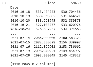
In this example, the code extracts the ‘Close’ column from the reliance DataFrame, calculates a 30 day Simple Moving Average (SMA) and then prints the refined DataFrame. This is a common step in financial analysis for computing technical indicators and identifying trends.
reliance = reliance['Close'].to_frame()
reliance['SMA30'] = reliance['Close'].rolling(30).mean()
reliance.dropna(inplace=True)

print(reliance)
Output:
Step 4: Plotting Simple Moving Averages
In this example, the code uses the plot() method to visualize the Close price along with the 30 day Simple Moving Average (SMA) from the reliance DataFrame.
reliance[['Close', 'SMA30']].plot(label='RELIANCE',
                                  figsize=(16, 8))
Output:

2. Exponential Moving Average (EMA) Using ewm()
The Exponential Moving Average (EMA) gives more weight to recent data points, making it more responsive to new changes compared to SMA. This makes EMA useful when recent movements are more important for analysis.
EMA places a greater weight and significance on the most recent data points. The formula to calculate EMA at the time period t is:
EMA_t =\begin{cases}x_0 & t = 0 \\\alpha x_t + (1 - \alpha) EMA_{t-1} & t > 0\end{cases}
where
In Python, EMA is calculated using .ewm() method. We can pass span or window as a parameter to .ewm(span = ) method.
Now we will be looking at an example to calculate EMA for a period of 30 days.
Step 1 and Step 2 will remain same.
Step 3: Isolates Column by Dataframe
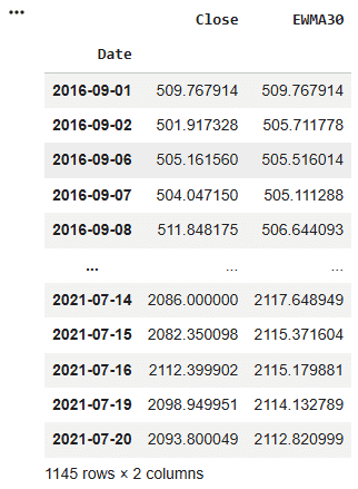
In this example the below code isolates the 'Close' column in the 'reliance' DataFrame, converts it into a DataFrame, computes the Exponential Moving Average (EWMA) with a span of 30 for the 'Close' column and prints the resulting DataFrame containing the EWMA values.
reliance = reliance['Close'].to_frame()

reliance['EWMA30'] = reliance['Close'].ewm(span=30).mean()

reliance
Output :
Step 4: Plotting Exponential Moving Averages
Here, code uses the plot() method to visualize the Close price and a 30 day Exponential Moving Average (EWMA) of the RELIANCE stock, displaying them on the same plot with a specified label and figure size.
reliance[['Close', 'EWMA30']].plot(label='RELIANCE',
                                   figsize=(16, 8))
Output :

3. Cumulative Moving Average (CMA) Using expanding()
To calculate the Cumulative Moving Average (CMA) in a Pandas DataFrame, we use the .expanding() function. This method computes the cumulative value of an aggregation function (such as .mean()) from the beginning up to the current point. CMA represents the average of all previous values up to time 𝑡. For data points
CMA_t = \frac{x_1 + x_2 + x_3 + \cdots + x_t}{t}
While calculating CMA we don't have any fixed size of the window. The size of the window keeps on increasing as time passes. In Python, we can calculate CMA using .expanding() method. Now we will see an example, to calculate CMA for a period of 30 days.
Step 1 and Step 2 will remain same.
Step 3: Transform Dataframe by Columns
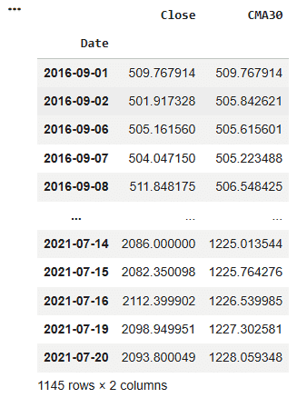
In this example, the code first extracts the ‘Close’ column from the reliance DataFrame and ensures it is in DataFrame format. It then calculates the Cumulative Moving Average (CMA) for the ‘Close’ prices using the expanding method. Finally, it prints the updated DataFrame containing the computed CMA values.
reliance = reliance['Close'].to_frame()

reliance['CMA30'] = reliance['Close'].expanding().mean()
reliance
Output:
Step 4: Plotting Cumulative Moving Averages
In this example code uses the .plot() method to visualize the 'Close' price and 30 day Cumulative Moving Average (CMA30) of Reliance stock, with the specified label and figure size.
reliance[['Close', 'CMA30']].plot(label='RELIANCE',
                                  figsize=(16, 8))
Output
