Probabilistic PCA and identification

I’ve been playing around with Bayesian Probabilistic PCA. Conceptually, the model is very simple, but the main problem with it is that while priors take care of location and scale invariance, by default the solutions are only unique up to an orthonormal rotation.

There has been a fair bit of discussion on this topic in this forum before, most notably in here which even resulted in an example in the library.

The conclusion reached there on the matter was from Chartl who proposed

Set loadings to lower-triangular (no more rotation invariance)
Set diagonal to positive (no more sign invariance)
Order diagonal (no more permutation invariance)

Thing is, this approach does no longer work for k>3 (which is easy to verify by setting k=5 in the example notebook).

I’ve been racking my brain and trying to find sources for this for the past few days and I think I figured it out, but I would like someone else to verify my reasoning. Hence the post.

The idea of forcing the matrix lower-triangular with positive diagonal elements seems to trace back to Geweke, Zhou 1996: “Measuring the Pricing Error of the Arbitrage Pricing Theory”. In reading the paper itself, however, there is an important yet easy to overlook caveat to their reasoning: namely, they assume that the weight matrix (f in their notation) is semi-orthonormal i.e. f @ f.T = I and that assumption is required in the theorem they use to show rotational invariance (end of pg10).

Now, from what I remember from my university linear algebra, to get an orthonormal matrix, you can start with any vector, then pick the next vector from the orthogonal space of the first vector as the second, then one from the orthogonal space of first two vectors as third and so on, i.e. you have one dimension of freedom less on each pick, effectively removing k(k-1)/2 degrees of freedom. Now forcing the matrix constructed that way to also be lower diagonal removes an additional k(k-1)/2 degrees. So it seems to me that instead of fixing k(k-1)/2 values for identification, one should actually fix twice that i.e. k(k-1).

I tested the library example with the following W construction:

def makeW2(d, k, dim_names):
    z = pm.HalfCauchy("W_z", 1.0, dims="latent_columns")
    L = pm.Cauchy("W_b", 0.0, 1.0, shape=(d-k,k), dims=("packed_dim",dim_names[1]))
    W = pm.Deterministic("W", pt.concatenate([pt.diag(z),L],axis=0), dims=dim_names)
    print(W.shape.eval(),L.shape.eval())
    return W

and that seems to work for k=4, k=5, meaning the chains converge and average rhat is 1.01. So the logic seems sound.

Granted, starting with a diagonal matrix in the weights, while identifying the model probably also skews the probability space by forcing first 3 questions all on separate factors. So it is definitely not ideal. So the question I have is: GZ96 seem to assume you can just sample orthonormal matrices without (at least seemingly) elaborating on how. Is there something obvious I am missing?
2 Likes

CC @aseyboldt maybe he has some ideas

From the footnote on page 10 of the linked paper, it looks like they generate weight matrices as follows:

    # This initial distribution is dealer's choice I think
    beta = pm.Normal('beta', dims=['latent_columns', 'latent_columns'])
    beta_posdef = beta @ beta.T
    L = pt.linalg.cholesky(beta_posdef)
    P = pt.linalg.solve(L, beta)
    beta_K = beta @ P.T

beta_K will always be lower triangular with positive diagonal. I didn’t see them mention orthonormality in their paper though. Etiher way, their setup differs somewhat because the vector of asset returns is a vector, and the factor matrix is observed data. The second point is not really important, but the first is. To adapt this method to the probabilistic PCA case, you’ll have to think about how to handle a non-square beta matrix. Something with SVD probably? That would get you two orthonomal square matrices from the weights, which seems to be a step in the right direction.

2 Likes

Thank you for the reply @jessegrabowski . But I think you skimmed the paper and missed that the pg 10 footnote is about the uniqueness of the orthonormal transformation P, not generating W.

Which is not to say I read the paper properly either. In re-reading it, I realised the only assumptions it makes on W (f) is E[W] = 0, E[W @ W.T] = I, and the reason he claims identification needs to be done w.r.t. orthonormal rotations is because orthronormal matrices are the class of matrices that preserve E[W @ W.T] value if W’ = P @ W, so it checks out.

I re-checked my code and realised that non-identification happened when k_true < k i.e. the model was forced to find a factor in the noise. In which case it makes sense it found multiple equally good options. Not something you are likely to see in real data where even the lower order components tend to have distinct enough eigenvalues up to pretty large values.

One thing I still don’t get is:

Order diagonal (no more permutation invariance)

Because in terms of matrices, permutations are also orthonormal so this seems completely unnecessary. Am I correct in this?

There are two approaches to this that can be easily automated with linear algebra packages:

  1. Take a standard normal matrix and do QR-decomposition and take the Q matrix, which will be uniformly distributed over orthonormal matrices. Because the space of orthonormal matrices is constrained, this will be a proper uniform distribution.

  2. Take a skew-symmetric matrix and apply matrix exponentiation. There I’m not sure what prior to put on the skew-symmetric matrix so that the resulting orthonormal is uniform.

Either way, you have to take care of the determinant (-1 gives you reflections, 1 gives you rotations, if I’m remembering correctly).

2 Likes

That 1. point is a really cool property @bob-carpenter! Any chance you can point me to a reference for it?

See, e.g.,

We have QR decomposition in pytensor but gradients aren’t implemented. This paper gives the procedure for LQ, which is just the transpose for QR. @Velochy if it’s something you want could you open an issue about it?

I don’t think so, at least not at this time. As you can see, the problem got solved without the need to actually create orthogonal matrices, so right now I don’t need the QR decomposition.

Thank you again for your help though!

In case anyone stumbles on this question:

There is actually a theoretically sound identification that is based on LQ decomposition.

To briefly sum it up: if we have a matrix of weights W and scores S, if W @ S is fixed, both W and S are unidentified up to scale, permutation, rotation and sign flip (as W can compensate for any change in S and vice versa). Putting normal priors on the elements of both gets rid of scale issues, but permutation, rotation and sign flips are still a thing.

However, if you take the LQ factorization of W so W = L @ Q, you end up with L @ Q @ W
Q is orthogonal, so we can just subsume it in S so S’ = Q @ S and if all elements of S are symmetrically distributed, it will not change the distribution.
L is lower triangular, and as D. Leung and M. Drton. Order-invariant prior specification in Bayesian factor analysis prove, if original W was i.i.d normal, then L is also i.i.d normal on the lower triangle and has Chi distribution (they don’t name it, but it is) on the diagonal.

So, with this, identification becomes very easy.

import pymc as pm, pytensor.tensor as pt
import numpy as np
import pymc_extras as pmx


# Output dimension, real dimension, factor dimension, number of samples
od,rd,fd,n = 10,7,5,300

# Create a dataset to test the FA
real_mat = np.random.normal(0,1,size=(rd,od))
real_scores = np.random.normal(0,1,size=(n,rd))
obs = real_scores @ real_mat + np.random.normal(0,0.1,size=(n,od))

with pm.Model() as model:

    # Create the W matrix
    tu_inds = np.triu_indices(n=fd,m=od,k=1)
    wvals = pm.Normal('wvals',size=len(tu_inds[0]))
    wdvals = pmx.Chi('wdvals',size=fd,nu=fd-np.arange(fd))
    W = pt.zeros((fd,od))
    W = pt.set_subtensor(W[tu_inds],wvals)
    W = pt.set_subtensor(W[np.arange(fd),np.arange(fd)],wdvals)
    pm.Deterministic('W',W)
    
    # Non-marginalized model that directly gives the scores
    scores = pm.Normal('scores', mu=0, sigma=1, shape=(n,fd))
    sd = pm.HalfNormal('sd',sigma=0.5)
    pm.Normal('obs', mu=scores @ W, sigma=sd, shape=(n,od), observed=obs)
    
    # Alt: Marginalized model that leaves scores implicit
    #pm.MvNormal('obs', mu=0, cov=W.T @ W + 0.1*pt.eye(od), shape=(n,od), observed=obs)

    idata = pm.sample(tune=2000)

And to check if all chains converged to the same solution:

import pandas as pd
from plotnine import *

pvals = np.swapaxes(idata.posterior.W.values,-1,-2)@random_map

# Create a random map into two dimensions
random_map = np.random.normal(0,1,size=(fd,2))

# Reshape pvals into longform dataframe with category columns
df_long = pd.DataFrame([
    {
        'chain': chain_idx,
        'point': point_idx,
        'x': pvals[chain_idx, draw_idx, point_idx, 0],
        'y': pvals[chain_idx, draw_idx, point_idx, 1]
    }
    for chain_idx in range(pvals.shape[0])
    for draw_idx in range(pvals.shape[1]) 
    for point_idx in range(pvals.shape[2])
])

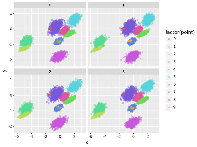
ggplot(df_long,aes(x='x',y='y',color='factor(point)')) + geom_point(alpha=0.3) + facet_wrap('~chain')

Usually, they do, and the result is:

1 Like

As for generating orthogonal (or semi-orthogonal) matrices, there also seems to be a rather clever way using Householder matrices that was proposed by Mezzadri 2007 and in theory also leads to identification, this time based on SVD rather than LQ decomposition, as was pointed out by Nirwan et al 2019.

In practice, that identification is a fair bit more involved, and I have yet to get it working properly (it samples, but ends up with all samples diverging about 70% of the time).

But in case someone needs a uniform distribution on (semi)orthogonal matrices for some other purposes, that approach seems very promising. I’m thinking of adding it to pymc_extras as my next PR :slight_smile:

There is one thing to look out for with the Leung-Drton identification. Namely, it is prone to last few factors getting switched from time to time. Here I ran the PCA for 32 times, and it is clearly visible here:

There is a dominant solution on 0,1,4,6,7,9,…
and then another pretty common option (2,5,8,18,19,…)
(along with numerous cases that had not yet converged in tuning)

There is an easy way to ameilorate this by initializing it with something close to the dominant solution by taking the QR decomposition of W, making sure it’s diagonal is positive and then taking it apart for initvals for both W itself and the scores.

qr = np.linalg.qr(mp['W'])
Q,R = qr.Q, qr.R
S = np.sign(np.diag(R))[:,None]
R *= S; Q*=S.T
tu_inds = np.triu_indices(n=fd,m=od,k=1)
wvals, wdvals = R[tu_inds], np.diag(R)
initvals = {'wvals':wvals, 'wdvals':wdvals, 'scores':mp['scores'] @ Q}

This does not fully fix it, but makes failure a lot less likely:

Realistically, if one needed things to be consistently converging well and identified, it seems that the best option would be to use an identification that only removes rotation, but leaves permutation and mirroring. This way, the geometry is probably the best behaved, as there are multiple high-density areas and any initial point is free to move fully to the closest one. And it is relatively easy to account for the sign flips and permutation in post-processing (permutation can be handled with Hungarian algorithm on the matrix of 1-abs(cosine distance) )

Again, these are mainly concerns for someone building a pipeline (like me). For one-off cases, it’s relatively easy to just run 20 chains and take the ones that converge to the dominant position.