Getting started with forecasting
You can define and configure forecasters in OpenSearch Dashboards by selecting Forecasting from the navigation panel.
Step 1: Define a forecaster
A forecaster represents a single forecasting task. You can create multiple forecasters to run in parallel, each analyzing a different data source. Follow these steps to define a new forecaster:
-
In the Forecaster list view, choose Create forecaster.
- Define the data source by entering the following information:
- Name – Provide a unique, descriptive name, such as
requests-10min. - Description – Summarize the forecaster’s purpose, for example,
Forecast total request count every 10 minutes. - Indexes – Select one or more indexes, index patterns, or aliases. Remote indexes are supported through cross-cluster search (
cluster-name:index-pattern). For more information, see Cross-cluster search. If the Security plugin is enabled, see Selecting remote indexes with fine-grained access control.
- Name – Provide a unique, descriptive name, such as
-
(Optional) Choose Add data filter to set a Field, Operator, and Value or choose Use query DSL to define a Boolean query. The following example uses a query domain-specific language (DSL) filter to match three URL paths:
{ "bool": { "should": [ { "term": { "urlPath.keyword": "/domain/{id}/short" } }, { "term": { "urlPath.keyword": "/sub_dir/{id}/short" } }, { "term": { "urlPath.keyword": "/abcd/123/{id}/xyz" } } ] } } -
Under Timestamp field, select the field that stores the timestamps.
-
In the Indicator (metric) section, add a metric for the forecaster. Each forecaster supports one metric for optimal accuracy. Choose one of the following options:
- Select a predefined aggregation:
average(),count(),sum(),min(), ormax(). - To use a custom aggregation, choose Custom expression under Forecast based on and define your own query DSL expression. For example, the following query forecasts the number of unique accounts with a specific account type:
{ "bbb_unique_accounts": { "filter": { "bool": { "must": [ { "wildcard": { "accountType": { "wildcard": "*blah*", "boost": 1 } } } ], "adjust_pure_negative": true, "boost": 1 } }, "aggregations": { "uniqueAccounts": { "cardinality": { "field": "account" } } } } } - Select a predefined aggregation:
-
(Optional) In the Categorical fields section, enable Split time series using categorical fields to generate forecasts at the entity level (for example, by IP address, product ID, or country code).
The number of unique entities that can be cached in memory is limited. Use the following formula to estimate capacity:
(data nodes × heap size × plugins.forecast.model_max_size_percent)
──────────────────────────────────────────────────────────────────
              entity-model size (MB)
For example, a cluster with 3 data nodes, each with 8 GB JVM heap and the default 10% model memory, would contain the following number of entities:
(8096 MB × 0.10 ÷ 1 MB) × 3 nodes ≈ 2429 entitiesTo determine the entity-model size, use the Profile Forecaster API. You can raise or lower the memory ceiling with the
plugins.forecast.model_max_size_percentsetting.
Forecasters cache models for the most frequently and recently observed entities, subject to available memory. Models for less common entities are loaded from indexes on a best-effort basis during each interval, with no guaranteed service-level agreement (SLA). Always validate memory usage against a representative workload.
For more information, see the blog post Improving Anomaly Detection: One Million Entities in One Minute. Although focused on anomaly detection, the recommendations apply to forecasting, as both features share the same underlying Random Cut Forest (RCF) model.
Step 2: Add model parameters
The Suggest parameters button in OpenSearch Dashboards initiates a review of recent history to recommend sensible defaults. You can override these defaults by adjusting the following parameters:
- Forecasting interval – Specifies the aggregation bucket (for example, 10 minutes). Longer intervals smooth out noise and reduce compute costs, but they delay detection. Shorter intervals detect changes sooner but increase resource usage and can introduce noise. Choose the shortest interval that still produces a stable signal.
- Window delay – Tells the forecaster how much of a delay to expect between event occurrence and ingestion. This delay adjusts the forecasting interval backward to ensure complete data coverage. For example, if the forecasting interval is 10 minutes and ingestion is delayed by 1 minute, setting the window delay to 1 minute ensures that the forecaster evaluates data from 1:49 to 1:59 rather than 1:50 to 2:00.
- To avoid missing data, set the window delay to the upper limit of the expected ingestion delay. However, longer delays reduce the real-time responsiveness of forecasts.
- Horizon – Specifies how many future buckets to predict. Forecast accuracy declines with distance, so choose only the forecast window that is operationally meaningful.
- History – Sets the number of historical data points used to train the initial (cold-start) model. The maximum is 10,000. More history improves initial model accuracy up to that limit.
The Advanced panel is collapsed by default, allowing most users to proceed with the suggested parameters. If you expand the panel, you can fine-tune three additional parameters: shingle size, suggested seasonality, and recency emphasis. These control how the forecaster balances recent fluctuations against long-term patterns.
Unless your data or use case demands otherwise, the defaults—shingle size 8, no explicit seasonality, and recency emphasis 2560—are reliable starting points.
Choosing a shingle size
Leave the Shingle size field empty to use the automatic heuristic:
- Start with the default value of 8.
- If Suggested seasonality is defined and greater than 16, replace it with half the season length.
- If Horizon is defined and one-third of the value is greater than the current candidate, update it accordingly.
The final value is the maximum of these three: max(8, seasonality ÷ 2, horizon ÷ 3)
If you provide a custom value, it overrides this calculation.
Determining storage amounts
By default, forecast results are stored in the opensearch-forecast-results index alias. You can:
- Build dashboards and visualizations.
- Connect the results to the Alerting plugin.
- Query the results as with any other OpenSearch index.
To manage storage, the plugin applies a rollover policy:
- Rollover trigger – When a primary shard reaches approximately 65 GB, a new backing index is created and the alias is updated.
- Retention – Rolled-over indexes are retained for at least 30 days before deletion.
You can customize this behavior using the following settings.
| Setting | Description | Default |
|---|---|---|
plugins.forecast.forecast_result_history_max_docs_per_shard | The maximum number of Lucene documents allowed per shard before triggering a rollover. One result is approximately 4 documents at around 47 bytes each, totaling about 65 GB. | 1_350_000_000 |
plugins.forecast.forecast_result_history_retention_period | The duration for which to retain forecast results. Supports duration formats such as 7d, 90d. | 30d |
Specifying a custom result index
You can store forecast results in a custom index by selecting Custom index and providing an alias name, such as abc. The plugin creates an alias like opensearch-forecast-result-abc that points to the backing index (for example, opensearch-forecast-result-abc-history-2024.06.12-000002).
To manage permissions, use hyphenated namespaces. For example, assign opensearch-forecast-result-financial-us-* to roles for the financial department’s us group. {: .note } If the Security plugin is enabled, ensure appropriate permissions are configured.
Flattening nested fields
If your custom result index’s documents include nested fields, enable the Flattened custom result index to simplify aggregation and visualization.
This creates a separate index prefixed with the custom index and forecaster name (for example, opensearch-forecast-result-abc-flattened-test) and attaches an ingest pipeline using a Painless script to flatten nested data.
If you later disable this option, the associated ingest pipeline is removed.
Use Index State Management to manage rollover and deletion of flattened result indexes.
Custom result index lifecycle management
The plugin triggers a rollover for custom result indexes when any of the following conditions are met.
| Parameter | Description | Type | Unit | Default | Required |
|---|---|---|---|---|---|
result_index_min_size | The minimum total primary shard size required to trigger a rollover. | Integer | MB | 51200 (50 GB) | No |
result_index_min_age | The minimum index age required to trigger a rollover. | Integer | Days | 7 | No |
result_index_ttl | The minimum amount of time before rolled-over indexes are deleted | Integer | Days | 60 | No |
Step 3: Test your forecaster
Backtesting is the fastest way to evaluate and refine key forecasting settings such as Interval and Horizon. During backtesting, the model is trained on historical data, generates forecasts, and plots them alongside actual values to help visualize prediction accuracy. If the results do not meet expectations, you can adjust the settings and run the test again.
Backtesting uses the following methods:
-
Training window: The model trains on historical data defined by the History setting.
-
Rolling forecast: The model progresses through the time series, repeatedly performing the following actions:
- Ingesting the next actual data point
- Emitting forecasts at each step
Because this is a retrospective simulation, forecasted values are plotted at their original timestamps, allowing you to see how well the model would have performed in real time.
Starting a backtest
To begin a test:
- Scroll to the bottom of the Add model parameters page.
- Select Create and test.
To skip testing and create the forecaster immediately, select Create.
Backtests usually take 1 or 2 minutes, but run time depends on the following factors.
| Factor | Why it matters |
|---|---|
| History length | More historical data increases training time. |
| Data density | Densely packed data slows aggregation. |
| Categorical field | The model trains separately for each entity. |
| Horizon | A longer forecast horizon increases the number of generated predictions. |
If the chart is empty, as shown in the following image, check that your index contains at least one time series with more than 40 data points at the selected interval.

Reading the chart
When the test succeeds, hover over any point on the chart to view exact values and confidence bounds:
- Actual data – Solid line
- Median prediction (P50) – Dotted line
- Confidence interval – Shaded band between P10 and P90
The following image shows the chart view.
Viewing forecasts from a specific date
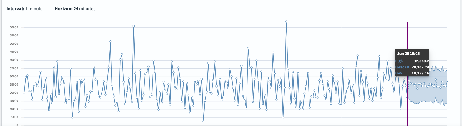
The forecast chart displays predictions starting from the final actual data point through the end of the configured horizon.
For example, you might configure the following settings in the Forecast from field:
- Last actual timestamp: Mar 5, 2025, 19:23
- Interval: 1 minute
- Horizon: 24
With these settings, the forecast range would span Mar 5, 2025, 19:23 – 19:47, as shown in the following image.

You can also use the Forecast from dropdown list to view forecasts from earlier test runs, as shown in the following image.

When you select an earlier Forecast from time, the forecast line is drawn directly over the historical data available at that moment. This causes the two series to overlap, as shown in the following image.

To return to the most recent forecast window, select Show latest.
Overlay mode: Side-by-side accuracy check
By default the chart displays forecasts that start from a single origin point. Toggle Overlay mode to lay a forecast curve directly on top of the actual series and inspect accuracy across the entire timeline.
Because the model emits one forecast per horizon step, for example, 24 forecasts when the horizon is 24, a single timestamp can have many forecasts that were generated from different origins. Overlay mode lets you decide which lead time (k) to plot:
- Horizon index 0 = Immediate next step
- Horizon index 1 = 1 step ahead
- Horizon index 23 = 23 steps ahead
The horizon control defaults to index 3, but you can choose any value to focus on a different lead time.
The following image shows Overlay mode enabled with a horizon index of 3. The visualization plots the forecast curve (in purple) directly on top of the actual data points (shown with white-filled markers). This lets you evaluate the accuracy of the model’s three-steps-ahead prediction across the full timeline. The forecast range is displayed as a shaded band around the predicted values, helping highlight uncertainty.

View multiple forecast series
A high-cardinality forecaster can display many time series at once. Use the Time series per page dropdown menu in the results panel to switch between the following views:
- Single-series view (default): Renders one entity per page for maximum readability.
- Multi-series view: Plots up to five entities side by side. Confidence bands are translucent by default—hover over a line to highlight its associated band.
Actual and forecast lines are overlaid so you can assess accuracy point by point. However, in Multi-series view, the overlapping lines can make the chart more difficult to interpret. To reduce visual clutter, go to Visualization options and turn off Show actual data at forecast.
The following image shows the chart with actual and forecast lines overlaid.

The following image shows the same chart with actual lines hidden at forecast time to simplify the view.

Exploring the timeline
Use the following timeline controls to navigate, magnify, and filter any span of your forecast history:
- Zoom – Select + / – to zoom in on forecasts or broaden context.
- Pan – Use the arrow buttons to move to earlier or later data points, if any.
- Quick Select – Choose common ranges, such as “Last 24 hours”, or supply custom dates for the result range.
Sorting options in multi-series view
When a forecaster tracks more than five entities, the chart can’t show every line at once.
In Multi-series view, you therefore choose the five most informative series and decide what “informative” means by selecting a sort method. The following table lists the available sort methods.
| Sort method | What it shows | When to use it |
|---|---|---|
| Minimum confidence-interval width (default) | The five series whose prediction bands are narrowest. A narrow band indicates that the model is highly certain about its forecast. | Surface the most “trustworthy” forecasts. |
| Maximum confidence-interval width | The five series with the widest bands—forecasts the model is least sure about. | Spot risky or noisy series that may need review or more training data. |
| Minimum value within the horizon | The lowest predicted point across the forecast window for each entity, sorted in ascending order. | Identify entities expected to drop the farthest—useful for capacity planning or alerting on potential dips. |
| Maximum value within the horizon | The highest predicted point across the horizon for each entity, sorted in descending order. | Highlight series with the greatest expected peaks, such as traffic spikes or sales surges. |
| Distance to threshold value | Filters forecasts by a numeric threshold (>, <, ≥, ≤) and then orders the remainder by how far they sit from that threshold. | Investigate entities that breach—or nearly breach—an SLA or business KPI, such as “show anything forecast to exceed 10,000 requests”. |
If the forecaster monitors five or fewer entities, Multi-series view displays all of them. When there are more than five, the view reranks them dynamically each time you change the sort method or adjust the threshold, ensuring that the most relevant series stay in focus.
To focus on a specific subset of entities, switch Filter by to Custom query and enter a query DSL query. The following example shows entities where the host equals server_1:
{
  "nested": {
    "path": "entity",
    "query": {
      "bool": {
        "must": [
          { "term":     { "entity.name":  "host"     } },
          { "wildcard": { "entity.value": "server_1" } }
        ]
      }
    }
  }
}
Next, select a sort method, such as Maximum value within the horizon, and select Update visualization. The chart updates to show only the forecast series for host:server_1, ranked according to your selected criteria.
Edit a forecaster
If the initial backtest shows weak performance, you can adjust the forecaster’s configuration and run the test again.
To edit a forecaster:
- Open the forecaster’s Details page and select Edit to enter edit mode.
- Modify the settings as needed—for example, add a Category field, change the Interval, or increase the History window.
-
Select Update. The validation panel automatically evaluates the new configuration and flags any issues.
The following image shows the validation process in progress.
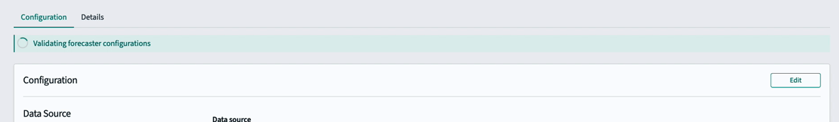
- Resolve any validation errors. When the panel becomes green, select Start test in the upper-right corner to run another backtest with the updated parameters.
Real-time forecasting
Once you are confident in the forecasting configuration, go to the Details page and click Start forecasting to begin real-time forecasting. The forecaster will generate new predictions at each interval moving forward.
A Live badge appears when the chart is synchronized with the most recent data.
Unlike backtesting, real-time forecasting continuously attempts to initialize using live data if there is not enough historical data. During this initialization period, the forecaster displays an initialization status until it has enough data to begin emitting forecasts.
Next steps
Once you have tested and refined your forecaster, you can begin using it to generate live forecasts or manage it over time. To learn how to start, stop, delete, or update an existing forecaster, see Managing forecasters.