Big O Notation Tutorial – A Guide to Big O Analysis
Last Updated :
21 Apr, 2025
Big O notation is a powerful tool used in computer science to describe the time complexity or space complexity of algorithms. Big-O is a way to express the upper bound of an algorithm’s time or space complexity.
- Describes the asymptotic behavior (order of growth of time or space in terms of input size) of a function, not its exact value.
- Can be used to compare the efficiency of different algorithms or data structures.
- It provides an upper limit on the time taken by an algorithm in terms of the size of the input. We mainly consider the worst case scenario of the algorithm to find its time complexity in terms of Big O
- It’s denoted as O(f(n)), where f(n) is a function that represents the number of operations (steps) that an algorithm performs to solve a problem of size n.

BIg O Definition
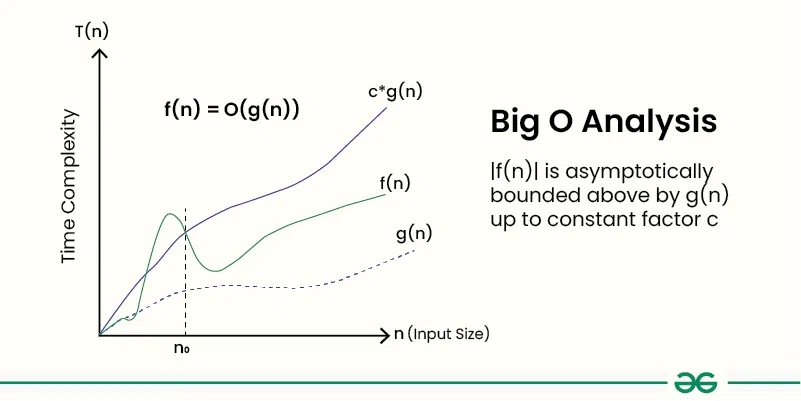
Given two functions f(n) and g(n), we say that f(n) is O(g(n)) if there exist constants c > 0 and n0 >= 0 such that f(n) <= c*g(n) for all n >= n0.
In simpler terms, f(n) is O(g(n)) if f(n) grows no faster than c*g(n) for all n >= n0 where c and n0 are constants.
Importance of Big O Notation
Big O notation is a mathematical notation used to find an upper bound on time taken by an algorithm or data structure. It provides a way to compare the performance of different algorithms and data structures, and to predict how they will behave as the input size increases.
Big O notation is important for several reasons:
- Big O Notation is important because it helps analyze the efficiency of algorithms.
- It provides a way to describe how the runtime or space requirements of an algorithm grow as the input size increases.
- Allows programmers to compare different algorithms and choose the most efficient one for a specific problem.
- Helps in understanding the scalability of algorithms and predicting how they will perform as the input size grows.
- Enables developers to optimize code and improve overall performance.
A Quick Way to find Big O of an Expression
- Ignore the lower order terms and consider only highest order term.
- Ignore the constant associated with the highest order term.
Example 1: f(n) = 3n2 + 2n + 1000Logn + 5000
After ignoring lower order terms, we get the highest order term as 3n2
After ignoring the constant 3, we get n2
Therefore the Big O value of this expression is O(n2)
Example 2 : f(n) = 3n3 + 2n2 + 5n + 1
Dominant Term: 3n3
Order of Growth: Cubic (n3)
Big O Notation: O(n3)
Properties of Big O Notation
Below are some important Properties of Big O Notation:
1. Reflexivity
For any function f(n), f(n) = O(f(n)).
Example:
f(n) = n2, then f(n) = O(n2).
2. Transitivity
If f(n) = O(g(n)) and g(n) = O(h(n)), then f(n) = O(h(n)).
Example:
If f(n) = n^2, g(n) = n^3, and h(n) = n^4, then f(n) = O(g(n)) and g(n) = O(h(n)).
Therefore, by transitivity, f(n) = O(h(n)).
3. Constant Factor
For any constant c > 0 and functions f(n) and g(n), if f(n) = O(g(n)), then cf(n) = O(g(n)).
Example:
f(n) = n, g(n) = n2. Then f(n) = O(g(n)). Therefore, 2f(n) = O(g(n)).
4. Sum Rule
If f(n) = O(g(n)) and h(n) = O(k(n)), then f(n) + h(n) = O(max( g(n), k(n) ) When combining complexities, only the largest term dominates.
Example:
f(n) = n2, h(n) = n3. Then , f(n) + h(n) = O(max(n2 + n3) = O ( n3)
5. Product Rule
If f(n) = O(g(n)) and h(n) = O(k(n)), then f(n) * h(n) = O(g(n) * k(n)).
Example:
f(n) = n, g(n) = n2, h(n) = n3, k(n) = n4. Then f(n) = O(g(n)) and h(n) = O(k(n)). Therefore, f(n) * h(n) = O(g(n) * k(n)) = O(n6).
6. Composition Rule
If f(n) = O(g(n)) and g(n) = O(h(n)), then f(g(n)) = O(h(n)).
Example:
f(n) = n2, g(n) = n, h(n) = n3. Then f(n) = O(g(n)) and g(n) = O(h(n)). Therefore, f(g(n)) = O(h(n)) = O(n3).
Common Big-O Notations
Big-O notation is a way to measure the time and space complexity of an algorithm. It describes the upper bound of the complexity in the worst-case scenario. Let’s look into the different types of time complexities:
1. Linear Time Complexity: Big O(n) Complexity
Linear time complexity means that the running time of an algorithm grows linearly with the size of the input.
For example, consider an algorithm that traverses through an array to find a specific element:
Code Snippet
bool findElement(int arr[], int n, int key)
{
    for (int i = 0; i < n; i++) {
        if (arr[i] == key) {
            return true;
        }
    }
    return false;
}
2. Logarithmic Time Complexity: Big O(log n) Complexity
Logarithmic time complexity means that the running time of an algorithm is proportional to the logarithm of the input size.
For example, a binary search algorithm has a logarithmic time complexity:
Code Snippet
int binarySearch(int arr[], int l, int r, int x)
{
    if (r >= l) {
        int mid = l + (r - l) / 2;
        if (arr[mid] == x)
            return mid;
        if (arr[mid] > x)
            return binarySearch(arr, l, mid - 1, x);
        return binarySearch(arr, mid + 1, r, x);
    }
    return -1;
}
3. Quadratic Time Complexity: Big O(n2) Complexity
Quadratic time complexity means that the running time of an algorithm is proportional to the square of the input size.
For example, a simple bubble sort algorithm has a quadratic time complexity:
Code Snippet
void bubbleSort(int arr[], int n)
{
    for (int i = 0; i < n - 1; i++) {
        for (int j = 0; j < n - i - 1; j++) {
            if (arr[j] > arr[j + 1]) {
                swap(&arr[j], &arr[j + 1]);
            }
        }
    }
}
4. Cubic Time Complexity: Big O(n3) Complexity
Cubic time complexity means that the running time of an algorithm is proportional to the cube of the input size.
For example, a naive matrix multiplication algorithm has a cubic time complexity:
Code Snippet
void multiply(int mat1[][N], int mat2[][N], int res[][N])
{
    for (int i = 0; i < N; i++) {
        for (int j = 0; j < N; j++) {
            res[i][j] = 0;
            for (int k = 0; k < N; k++)
                res[i][j] += mat1[i][k] * mat2[k][j];
        }
    }
}
5. Polynomial Time Complexity: Big O(nk) Complexity
Polynomial time complexity refers to the time complexity of an algorithm that can be expressed as a polynomial function of the input size n. In Big O notation, an algorithm is said to have polynomial time complexity if its time complexity is O(nk), where k is a constant and represents the degree of the polynomial.
Algorithms with polynomial time complexity are generally considered efficient, as the running time grows at a reasonable rate as the input size increases. Common examples of algorithms with polynomial time complexity include linear time complexity O(n), quadratic time complexity O(n2), and cubic time complexity O(n3).
6. Exponential Time Complexity: Big O(2n) Complexity
Exponential time complexity means that the running time of an algorithm doubles with each addition to the input data set.
For example, the problem of generating all subsets of a set is of exponential time complexity:
Code Snippet
void generateSubsets(int arr[], int n)
{
    for (int i = 0; i < (1 << n); i++) {
        for (int j = 0; j < n; j++) {
            if (i & (1 << j)) {
                cout << arr[j] << " ";
            }
        }
        cout << endl;
    }
}
7. Factorial Time Complexity: Big O(n!) Complexity
Factorial time complexity means that the running time of an algorithm grows factorially with the size of the input. This is often seen in algorithms that generate all permutations of a set of data.
Here’s an example of a factorial time complexity algorithm, which generates all permutations of an array:
Code Snippet
void permute(int* a, int l, int r)
{
    if (l == r) {
        for (int i = 0; i <= r; i++) {
            cout << a[i] << " ";
        }
        cout << endl;
    }
    else {
        for (int i = l; i <= r; i++) {
            swap(a[l], a[i]);
            permute(a, l + 1, r);
            swap(a[l], a[i]); // backtrack
        }
    }
}
If we plot the most common Big O notation examples, we would have graph like this:

Mathematical Examples of Runtime Analysis
Below table illustrates the runtime analysis of different orders of algorithms as the input size (n) increases.
| n | log(n) | n | n * log(n) | n^2 | 2^n | n! |
|---|
| 10 | 1 | 10 | 10 | 100 | 1024 | 3628800 |
| 20 | 2.996 | 20 | 59.9 | 400 | 1048576 | 2.432902e+1818 |
Algorithmic Examples of Runtime Analysis
Below table categorizes algorithms based on their runtime complexity and provides examples for each type.
| Type | Notation | Example Algorithms |
|---|
| Logarithmic | O(log n) | Binary Search |
| Linear | O(n) | Linear Search |
| Superlinear | O(n log n) | Heap Sort, Merge Sort |
| Polynomial | O(n^c) | Strassen’s Matrix Multiplication, Bubble Sort, Selection Sort, Insertion Sort, Bucket Sort |
| Exponential | O(c^n) | Tower of Hanoi |
| Factorial | O(n!) | Determinant Expansion by Minors, Brute force Search algorithm for Traveling Salesman Problem |
Algorithm Classes with Number of Operations
Below are the classes of algorithms and their number of operations assuming that there are no constants.
Big O Notation Classes
| f(n)
| Big O Analysis (number of operations) for n = 10
|
|---|
constant
| O(1)
| 1
|
|---|
logarithmic
| O(logn)
| 3.32
|
|---|
linear
| O(n)
| 10
|
|---|
O(nlogn)
| O(nlogn)
| 33.2
|
|---|
quadratic
| O(n2)
| 102
|
|---|
cubic
| O(n3)
| 103
|
|---|
exponential
| O(2n)
| 1024
|
|---|
factorial
| O(n!)
| 10!
|
|---|
Comparison of Big O Notation, Big Ω (Omega) Notation, and Big θ (Theta) Notation
Below is a table comparing Big O notation, Ω (Omega) notation, and θ (Theta) notation:
| Notation | Definition | Explanation |
|---|
| Big O (O) | f(n) ≤ C * g(n) for all n ≥ n0 | Describes the upper bound of the algorithm’s running time. Used most of the time. |
| Ω (Omega) | f(n) ≥ C * g(n) for all n ≥ n0 | Describes the lower bound of the algorithm’s running time . Used less |
| θ (Theta) | C1 * g(n) ≤ f(n) ≤ C2 * g(n) for n ≥ n0 | Describes both the upper and lower bounds of the algorithm’s running time. Also used a lot more and preferred over Big O if we can find an exact bound. |
In each notation:
- f(n) represents the function being analyzed, typically the algorithm’s time complexity.
- g(n) represents a specific function that bounds f(n).
- C, C1, and C2 are constants.
- n0 is the minimum input size beyond which the inequality holds.
These notations are used to analyze algorithms based on their worst-case (Big O), best-case (Ω), and average-case (θ) scenarios.
Related Article:
Similar Reads
Analysis of Algorithms
Analysis of Algorithms is a fundamental aspect of computer science that involves evaluating performance of algorithms and programs. Efficiency is measured in terms of time and space. Basics on Analysis of Algorithms:Why is Analysis Important?Order of GrowthAsymptotic Analysis Worst, Average and Best
1 min read
Complete Guide On Complexity Analysis - Data Structure and Algorithms Tutorial
Complexity analysis is defined as a technique to characterise the time taken by an algorithm with respect to input size (independent from the machine, language and compiler). It is used for evaluating the variations of execution time on different algorithms. What is the need for Complexity Analysis?
15+ min read
Why is Analysis of Algorithm important?
Why is Performance of Algorithms Important ? There are many important things that should be taken care of, like user-friendliness, modularity, security, maintainability, etc. Why worry about performance? The answer to this is simple, we can have all the above things only if we have performance. So p
2 min read
Types of Asymptotic Notations in Complexity Analysis of Algorithms
We have discussed Asymptotic Analysis, and Worst, Average, and Best Cases of Algorithms. The main idea of asymptotic analysis is to have a measure of the efficiency of algorithms that don't depend on machine-specific constants and don't require algorithms to be implemented and time taken by programs
8 min read
Worst, Average and Best Case Analysis of Algorithms
In the previous post, we discussed how Asymptotic analysis overcomes the problems of the naive way of analyzing algorithms. Now let us learn about What is Worst, Average, and Best cases of an algorithm: 1. Worst Case Analysis (Mostly used) In the worst-case analysis, we calculate the upper bound on
10 min read
Asymptotic Analysis
Given two algorithms for a task, how do we find out which one is better? One naive way of doing this is - to implement both the algorithms and run the two programs on your computer for different inputs and see which one takes less time. There are many problems with this approach for the analysis of
3 min read
How to Analyse Loops for Complexity Analysis of Algorithms
We have discussed Asymptotic Analysis, Worst, Average and Best Cases and Asymptotic Notations in previous posts. In this post, an analysis of iterative programs with simple examples is discussed. The analysis of loops for the complexity analysis of algorithms involves finding the number of operation
15+ min read
Sample Practice Problems on Complexity Analysis of Algorithms
Prerequisite: Asymptotic Analysis, Worst, Average and Best Cases, Asymptotic Notations, Analysis of loops. Problem 1: Find the complexity of the below recurrence: { 3T(n-1), if n>0,T(n) = { 1, otherwise Solution: Let us solve using substitution. T(n) = 3T(n-1) = 3(3T(n-2)) = 32T(n-2) = 33T(n-3) .
15 min read
Basics on Analysis of Algorithms
Why is Analysis of Algorithm important?
Why is Performance of Algorithms Important ? There are many important things that should be taken care of, like user-friendliness, modularity, security, maintainability, etc. Why worry about performance? The answer to this is simple, we can have all the above things only if we have performance. So p
2 min read
Asymptotic Analysis
Given two algorithms for a task, how do we find out which one is better? One naive way of doing this is - to implement both the algorithms and run the two programs on your computer for different inputs and see which one takes less time. There are many problems with this approach for the analysis of
3 min read
Worst, Average and Best Case Analysis of Algorithms
In the previous post, we discussed how Asymptotic analysis overcomes the problems of the naive way of analyzing algorithms. Now let us learn about What is Worst, Average, and Best cases of an algorithm: 1. Worst Case Analysis (Mostly used) In the worst-case analysis, we calculate the upper bound on
10 min read
Types of Asymptotic Notations in Complexity Analysis of Algorithms
We have discussed Asymptotic Analysis, and Worst, Average, and Best Cases of Algorithms. The main idea of asymptotic analysis is to have a measure of the efficiency of algorithms that don't depend on machine-specific constants and don't require algorithms to be implemented and time taken by programs
8 min read
How to Analyse Loops for Complexity Analysis of Algorithms
We have discussed Asymptotic Analysis, Worst, Average and Best Cases and Asymptotic Notations in previous posts. In this post, an analysis of iterative programs with simple examples is discussed. The analysis of loops for the complexity analysis of algorithms involves finding the number of operation
15+ min read
How to analyse Complexity of Recurrence Relation
The analysis of the complexity of a recurrence relation involves finding the asymptotic upper bound on the running time of a recursive algorithm. This is usually done by finding a closed-form expression for the number of operations performed by the algorithm as a function of the input size, and then
7 min read
Introduction to Amortized Analysis
Amortized Analysis is used for algorithms where an occasional operation is very slow, but most other operations are faster. In Amortized Analysis, we analyze a sequence of operations and guarantee a worst-case average time that is lower than the worst-case time of a particularly expensive operation.
10 min read
Asymptotic Notations
Big O Notation Tutorial - A Guide to Big O Analysis
Big O notation is a powerful tool used in computer science to describe the time complexity or space complexity of algorithms. Big-O is a way to express the upper bound of an algorithm’s time or space complexity. Describes the asymptotic behavior (order of growth of time or space in terms of input si
10 min read
Big O vs Theta Θ vs Big Omega Ω Notations
1. Big O notation (O): It defines an upper bound on order of growth of time taken by an algorithm or code with input size. Mathematically, if f(n) describes the running time of an algorithm; f(n) is O(g(n)) if there exist positive constant C and n0 such that, 0 <= f(n) <= Cg(n) for all n >=
3 min read
Examples of Big-O analysis
Prerequisite: Analysis of Algorithms | Big-O analysis In the previous article, the analysis of the algorithm using Big O asymptotic notation is discussed. In this article, some examples are discussed to illustrate the Big O time complexity notation and also learn how to compute the time complexity o
13 min read
Difference between big O notations and tilde
In asymptotic analysis of algorithms we often encounter terms like Big-Oh, Omega, Theta and Tilde, which describe the performance of an algorithm. You can refer to the following links to get more insights about asymptotic analysis : Analysis of Algorithms Different NotationsDifference between Big Oh
4 min read
Analysis of Algorithms | Big-Omega Ω Notation
In the analysis of algorithms, asymptotic notations are used to evaluate the performance of an algorithm, in its best cases and worst cases. This article will discuss Big-Omega Notation represented by a Greek letter (Ω). Table of Content What is Big-Omega Ω Notation?Definition of Big-Omega Ω Notatio
9 min read
Analysis of Algorithms | Θ (Theta) Notation
In the analysis of algorithms, asymptotic notations are used to evaluate the performance of an algorithm by providing an exact order of growth. This article will discuss Big - Theta notations represented by a Greek letter (Θ). Definition: Let g and f be the function from the set of natural numbers t
6 min read