Bidirectional Search in AI

Bidirectional search in AI is an algorithm that searches simultaneously from both the initial state and the goal state, meeting in the middle to reduce search time. The aim of the article is to provide an in-depth understanding of the bidirectional search algorithm, its working mechanism, benefits and practical applications in artificial intelligence.

Understanding Bidirectional Search Algorithm

Bidirectional search is an effective search technique used in the field of artificial intelligence (AI) for finding the shortest path between an initial and a goal state. It operates by simultaneously running two separate search processes one forward from the initial state and the other backward from the goal state. The search stops when the two processes meet in the middle. This method is particularly useful in large search spaces where traditional search techniques like Depth-First Search (DFS) or Breadth-First Search (BFS) may be inefficient.

How Bidirectional Search Works?

Bidirectional search uses two simultaneous searches to potentially reduce the total search time. Here’s a step-by-step breakdown of how it typically works:

1. Initial Setup: Initialize two searches. One starts from the initial state and expands forward. The other starts from the goal state and expands backward.
2. Node Expansion: Both searches alternately expand the nearest unexplored node. For each node, all possible successors (in the forward direction) or predecessors (in the backward direction) are generated.
3. Checking Intersections: After each expansion, check if any of the newly generated nodes are present in the frontier of the opposite search.
4. Meeting Point: Once a common node is discovered, this node acts as the meeting point and the optimal path can be constructed by joining the paths from the initial state to the meeting point and from the meeting point to the goal state.

Bidirectional Search for Maze Navigation

Step 1: Import Necessary Libraries

This step includes importing libraries needed for the code such as matplotlib for visualization, numpy for array manipulation and collections.deque for implementing a double-ended queue.

import matplotlib.pyplot as plt
import numpy as np
from collections import deque

Step 2: Define a Function to Check Valid Moves

This function checks whether a given move within the maze is valid. A move is considered valid if it is within the maze bounds and the maze cell is not a wall (1).

def is_valid_move(x, y, maze):
    return 0 <= x < len(maze) and 0 <= y < len(maze[0]) and maze[x][y] == 0

Step 3: Define a Breadth-First Search (BFS) Function

The BFS function explores the maze in four directions (up, down, left, right) from the current position. It updates the queue, visited nodes and parent mapping for path reconstruction later.

def bfs(queue, visited, parent):
    (x, y) = queue.popleft()
    directions = [(-1, 0), (1, 0), (0, -1), (0, 1)]  # Up, Down, Left, Right moves
    for dx, dy in directions:
        nx, ny = x + dx, y + dy
        if is_valid_move(nx, ny, maze) and (nx, ny) not in visited:
            queue.append((nx, ny))
            visited.add((nx, ny))
            parent[(nx, ny)] = (x, y)

Step 4: Implement Bidirectional Search Algorithm

In this step, two BFS searches are initiated from both the start and goal points. The two searches continue until they meet at a common point (intersection). If an intersection is found, it returns the intersection node and the paths from both directions.

def bidirectional_search(maze, start, goal):
    if maze[start[0]][start[1]] == 1 or maze[goal[0]][goal[1]] == 1:
        return None, None, None
    
    queue_start = deque([start])
    queue_goal = deque([goal])
    visited_start = set([start])
    visited_goal = set([goal])
    parent_start = {start: None}
    parent_goal = {goal: None}
    
    while queue_start and queue_goal:
        bfs(queue_start, visited_start, parent_start)
        bfs(queue_goal, visited_goal, parent_goal)
        
        # Check for intersection
        intersect_node = None
        for node in visited_start:
            if node in visited_goal:
                intersect_node = node
                break
        
        if intersect_node is not None:
            return (intersect_node, parent_start, parent_goal)
    
    return (None, None, None)

Step 5: Reconstruct the Path from Start to Goal

This function reconstructs the final path by backtracking from the intersection node. It combines the path from start to the intersection and from the intersection to the goal.

def reconstruct_path(intersect_node, parent_start, parent_goal):
    if intersect_node is None:
        return []
    
    path = []
    # from start to intersection
    step = intersect_node
    while step is not None:
        path.append(step)
        step = parent_start[step]
    path.reverse()
    
    # from intersection to goal
    step = parent_goal[intersect_node]
    while step is not None:
        path.append(step)
        step = parent_goal[step]
    
    return path

Step 6: Visualize the Maze and the Path

This function visualizes the maze and the solution path using matplotlib. It plots the maze cells, the solution path (in gold), the start point (green) and the goal point (red).

def visualize(maze, path, start, goal):
    maze_copy = np.array(maze)
    fig, ax = plt.subplots(figsize=(10, 10))
    
    # Coloring the maze
    cmap = plt.cm.Dark2
    colors = {'empty': 0, 'wall': 1, 'path': 2}
    for y in range(len(maze)):
        for x in range(len(maze[0])):
            color = 'white' if maze[y][x] == 0 else 'black'
            ax.fill_between([x, x+1], y, y+1, color=color)

    # Drawing the path
    if path:
        for (y, x) in path:
            ax.fill_between([x, x+1], y, y+1, color='gold', alpha=0.5)
    
    # Mark start and goal
    sy, sx = start
    gy, gx = goal
    ax.plot(sx+0.5, sy+0.5, 'go')  # green dot at start
    ax.plot(gx+0.5, gy+0.5, 'ro')  # red dot at goal

    # Set limits and grid
    ax.set_xlim(0, len(maze[0]))
    ax.set_ylim(0, len(maze))
    ax.set_xticks(range(len(maze[0])))
    ax.set_yticks(range(len(maze)))
    ax.grid(which='both')
    ax.invert_yaxis()  # Invert the y-axis so the first row is at the top
    ax.xaxis.tick_top()  # and the x-axis is on the top

    plt.show()

Step 7: Define the Maze, Start and Goal Points

This step sets up the maze layout and the start and goal points.

# Define the maze
maze = [
    [0, 1, 0, 0, 0],
    [0, 1, 0, 1, 0],
    [0, 0, 0, 1, 0],
    [0, 1, 0, 0, 0],
    [0, 0, 0, 1, 0]
]

start = (0, 0)
goal = (4, 4)

Step 8: Run the Bidirectional Search, Reconstruct Path and Visualize

Finally, the code runs the bidirectional search, reconstructs the path if found and visualizes it using the previously defined functions.

intersect_node, parent_start, parent_goal = bidirectional_search(maze, start, goal)
path = reconstruct_path(intersect_node, parent_start, parent_goal)
visualize(maze, path, start, goal)

Output:

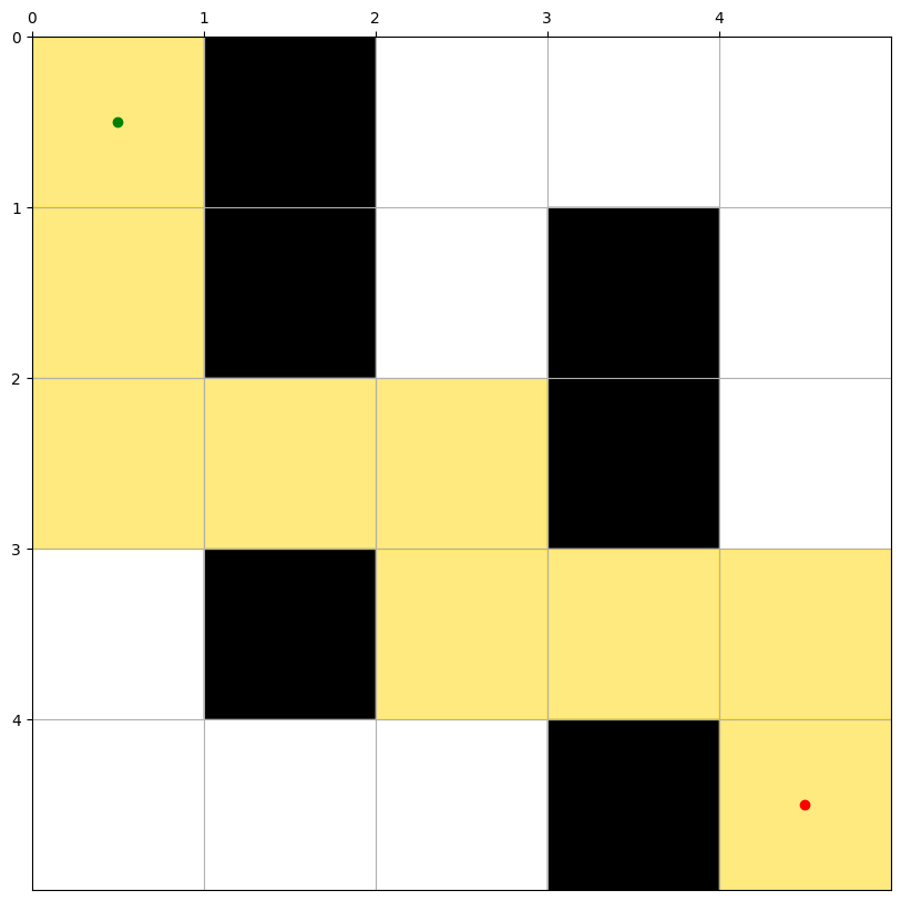
The output graph represents the path from the starting point to the goal point.

Practical Applications of Bidirectional Search in AI

Bidirectional search is not just a theoretical construct but has practical applications in various fields within AI:

• Pathfinding in AI Navigation Systems: Commonly used in scenarios ranging from GPS navigation to movement planning in robotics.
• Puzzle Solving: Effective in games and puzzle-solving where a clear goal state is defined, such as in solving Rubik's Cube.
• Network Analysis: Useful in social network analysis, where connections between entities (like finding the degree of separation between two people) need to be established quickly.

Benefits of Bidirectional Search

• Efficiency: The most notable advantage is its speed. By simultaneously searching from both ends towards the middle, it reduces the search space dramatically, often leading to quicker results.
• Optimality: When used with uniform-cost search strategies, bidirectional search is guaranteed to find an optimal solution if one exists.
• Reduced Memory Footprint: It often requires less memory than traditional algorithms like BFS, especially in densely connected graphs or large search spaces.

Challenges and Considerations

• Implementation Complexity: Managing two simultaneous searches and ensuring they meet optimally can be complex compared to unidirectional strategies.
• Memory Management: While generally less memory-intensive than some alternatives, bidirectional search still requires careful management of both search frontiers.
• Applicability: It's not suitable for all problems. For instance, it's most effective in searchable spaces where both forward and backward expansion are feasible and meaningful.