Exponential Smoothing for Time Series Forecasting
Last Updated :
25 Aug, 2025
Exponential smoothing is a popular time series forecasting method known for its simplicity and accuracy in predicting future trends based on historical data. It assumes that future patterns will be similar to recent past data and focuses on learning the average demand level over time.
It gives more weight to the most recent observations and reduces exponentially as the distance from the observations rises with the premise that the future will be similar to the recent past. The word "exponential smoothing" refers to the fact that each demand observation is assigned an exponentially diminishing weight.
- This technique captures the general pattern and can be expanded to include trends and seasonal variations, allowing for precise time series forecasts using past data.
- This method gives a bit of erroneous long-term forecasts.
- It works well with the technique of smoothing when the parameters of the time series change gradually over time.
Types of Exponential Smoothing
Exponential smoothing forecasting can be divided into three main types:
1. Simple or Single Exponential Smoothing
Simple Smoothing is a forecasting method used for time series data that does not exhibit a trend or seasonality. It relies on univariate data and uses a single parameter called alpha (\alpha) or the smoothing factor.
Key points:
- \alpha determines how much weight is given to the current observation versus the past estimates.
- A smaller \alpha gives more importance to past predictions, while a larger \alpha emphasizes recent observations.
- The value of \alpha typically ranges from 0 to 1.
The smoothing process balances past and present data to provide more stable forecasts. The formula for simple smoothing is as follows:
s_t = \alpha x_t + (1 - \alpha) s_{t-1} = s_{t-1} + \alpha (x_t - s_{t-1})
Where:
- s_t = smoothed statistic (simple weighted average of current observation x_t)
- s_{t-1} = previous smoothed statistic
- \alpha = smoothing factor of data; 0 < \alpha < 1
- t = time period
2. Double Exponential Smoothing
Double Exponential Smoothing, also called Holt’s Trend Model, second-order smoothing or Holt’s Linear Smoothing which is a method used to forecast the trend of a time series that does not have seasonality.
- It accounts for trends in the data by introducing a trend component.
- It uses alpha \alpha to smooth the level of the series.
- It uses beta \beta to smooth the trend or rate of change.
- It supports both additive and multiplicative trends.
Double exponential smoothing works better than simple smoothing when a time series shows a trend but no seasonal pattern.
The formulas for Double exponential smoothing are as follows:
s_t = \alpha x_t + (1 - \alpha)(s_{t-1} + b_{t-1})
\beta_t = \beta (s_t - s_{t-1}) + (1 - \beta) b_{t-1}
Where:
- b_t = best estimate of the trend at time t
- \beta = trend smoothing factor; 0 < \beta <1
3. Holt-Winters’ Exponential Smoothing
Triple exponential smoothing (also known as Holt-Winters smoothing) is a smoothing method used to predict time series data with both a trend and seasonal component. New smoothing parameter, gamma (\gamma), is used to control the effect of seasonal component.
The technique uses exponential smoothing applied three times:
- (\alpha) the level (intercept),
- (\beta) the trend and
- (\gamma) the seasonal component.
This method can be divided into two categories, depending on the seasonality.
- Holt-Winter’s Additive Method (HWIM) is used for addictive seasonality.
- Holts-Winters Multiplicative method (MWM) is used for multiplicative seasonality.
The formulas for the triple exponential smoothing are as follows:
s_{0} = x_{0}
s_t = \alpha (x_t/c_{t - L}) +(1- \alpha)(s_{t-1} +b_{t-1})
b_t = \beta(s_t -s_{t - 1} )+(1- \beta)b_{t-1}
c_t = \gamma x_t/s_t + (1 - \gamma) c_{t-L}
Where:
- s_t = smoothed statistic
- s_{t-1} = previous smoothed statistic
- \alpha = smoothing factor of data (0 <\alpha < 1)
- t = time period
- b_t = best estimate of a trend at time t
- \beta = trend smoothing factor (0 < \beta <1)
- c_t = seasonal component at time t
- \gamma = seasonal smoothing parameter (0 < \gamma < 1)
The Holt-Winters method is the most precise of the three, but it is also the most complicated. It involves more data and more calculations than the others.
Implementation of Exponential Smoothing
We will be implementing different types of smoothing methods using python programming language. We are going to use a dataset called AirPassengers which is a time-series dataset that includes the monthly passenger numbers of airlines in the years 1949 to 1960.
1. Importing Libraries
We will import pandas and matplotlib library.
Python
import pandas as pd
import matplotlib.pyplot as plt
2. Loading the Dataset
We will now load the AirPassengers dataset and inspect the first few rows.
Dataset download link: AirPassengers.csv
- pd.read_csv(): Reads the CSV file into a pandas DataFrame.
- parse_dates=['Month']: Converts the 'Month' column to a datetime format while loading the data.
- index_col='Month': Sets the 'Month' column as the index of the DataFrame.
- data.head(): Displays the first five rows of the dataset.
Python
data = pd.read_csv('AirPassengers.csv', parse_dates=['Month'], index_col='Month')
data.head()
Output:
 AirPassengers Dataset
3. Visualizing the Data
We will now plot the dataset and visualize the number of passengers over time.
- plt.plot(data): Plots the data.
- plt.xlabel('Year'): Labels the x-axis as "Year" to represent the time dimension of the dataset.
- plt.ylabel('Number of Passengers'): Labels the y-axis as "Number of Passengers" to indicate the metric being plotted.
- plt.show(): Displays the plot to visualize the data.
Python
plt.plot(data)
plt.xlabel('Year')
plt.ylabel('Number of Passengers')
plt.show()
Output:
 Visualizing the Data
We can see that the number of passengers appears to be increasing over time, with some seasonality as well.
4. Appling Single Exponential smoothing
We will now apply simple exponential smoothing to the dataset using statsmodels library.
- SimpleExpSmoothing(data): Initializes the Simple Exponential Smoothing model using the dataset data.
- model.fit(): Fits the model to the data, generating the smoothed values based on the provided dataset.
Python
from statsmodels.tsa.api import SimpleExpSmoothing
model = SimpleExpSmoothing(data)
model_single_fit = model.fit()
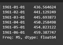
4.1. Making predictions
We will now forecast the next 6 time periods using the fitted model.
- model_single_fit.forecast(6): Generates a forecast for the next 6 periods based on the fitted Simple Exponential Smoothing model.
Python
forecast_single = model_single_fit.forecast(6)
print(forecast_single)
Output:
 Single Exponential smoothing
4.2. Visualizing Single Exponential Smoothing
We will now visualize the original data, fitted values and the forecasted values for the next 40 periods.
- model_single_fit.forecast(40): Forecasts the next 40 periods using the fitted model.
- plt.plot(data, label='Original Data'): Plots the original dataset (number of passengers) with the label "Original Data".
- plt.plot(model_single_fit.fittedvalues, label='Fitted Values'): Plots the fitted values (smoothed data) from the model with the label "Fitted Values".
- plt.plot(forecast_single, label='Forecast'): Plots the forecasted values for the next 40 periods with the label "Forecast".
- plt.legend(): Displays the legend to differentiate between the original data, fitted values and forecast.
- plt.show(): Displays the plot for visualization.
Python
forecast_single = model_single_fit.forecast(40)
plt.plot(data, label='Original Data')
plt.plot(model_single_fit.fittedvalues, label='Fitted Values')
plt.plot(forecast_single, label='Forecast')
plt.xlabel('Year')
plt.ylabel('Number of Passengers')
plt.title('Single Exponential Smoothing')
plt.legend()
plt.show()
Output:
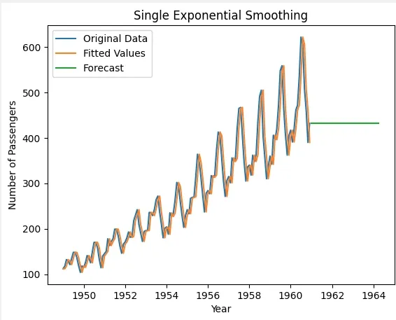 Visualizing Single Exponential Smoothing
5. Appling Double Exponential Smoothing
We will now apply Holt's linear trend method to the dataset for double exponential smoothing using statsmodels library.
- Holt(data): Initializes the Holt's linear trend model using the dataset data.
- model_double.fit(): Fits the model to the data, capturing both level and trend in the series.
Python
from statsmodels.tsa.api import Holt

model_double = Holt(data)
model_double_fit = model_double.fit()
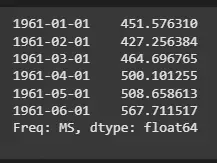
5.1. Making Predictions
We will now forecast the next 6 time periods using Holt's linear trend model.
- model_double_fit.forecast(6): Generates a forecast for the next 6 periods based on the fitted Holt's model, which includes both level and trend.
Python
forecast_double = model_double_fit.forecast(6)
print(forecast_double)
Output:
 Double Exponential Smoothing
5.2. Visualizing Double Exponential Smoothing
We will now visualize the original data, fitted values and forecasted values for the next 40 periods using Holt's method.
- model_double_fit.forecast(40): Forecasts the next 40 periods using the fitted Holt's linear trend model.
- plt.plot(data, label='Original Data'): Plots the original dataset (number of passengers) with the label "Original Data".
- plt.plot(model_double_fit.fittedvalues, label='Fitted Values'): Plots the fitted values from the model with the label "Fitted Values".
- plt.plot(forecast_double, label='Forecast'): Plots the forecasted values for the next 40 periods with the label "Forecast".
Python
forecast_double = model_double_fit.forecast(40)
plt.plot(data, label='Original Data')
plt.plot(model_double_fit.fittedvalues, label='Fitted Values')
plt.plot(forecast_double, label='Forecast')
plt.xlabel('Year')
plt.ylabel('Number of Passengers')
plt.title('Double Exponential Smoothing')
plt.legend()
plt.show()
Output:
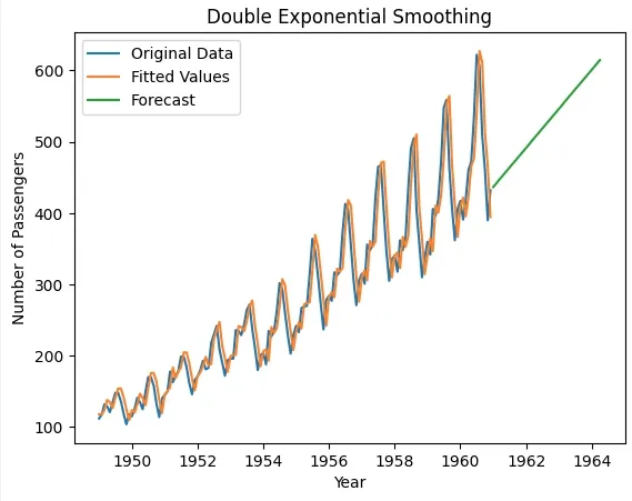 Visualizing Double Exponential Smoothing
6. Appling Holt-Winter’s Seasonal Smoothing
We will now apply triple exponential smoothing (Holt-Winters) to the dataset, accounting for seasonality, trend and level using statsmodels library.
- ExponentialSmoothing(): Initializes the Exponential Smoothing model
- seasonal_periods=12: Specifies a seasonal cycle of 12 periods (e.g., monthly data with yearly seasonality).
- trend='add': Specifies an additive trend component.
- seasonal='add': Specifies an additive seasonal component.
- model_triple.fit(): Fits the model to the data, incorporating the level, trend and seasonality.
Python
from statsmodels.tsa.api import ExponentialSmoothing

model_triple = ExponentialSmoothing(
    data,
    seasonal_periods=12,
    trend='add',
    seasonal='add')

model_triple_fit = model_triple.fit()
6.1. Making Predictions
We will now forecast the next 6 time periods using the fitted triple exponential smoothing model.
- model_triple_fit.forecast(6): Generates a forecast for the next 6 periods based on the fitted model.
Python
forecast_triple = model_triple_fit.forecast(6)
print(forecast_triple)
Output:
 Holt-Winter’s Seasonal Smoothing
6.2. Visualizing Triple Exponential Smoothing
We will now visualize the original data, fitted values and forecasted values for the next 40 periods using triple exponential smoothing.
- forecast_triple = model_triple_fit.forecast(40): Forecasts the next 40 periods using the fitted triple exponential smoothing model.
- plt.plot(data, label='Original Data'): Plots the original dataset (number of passengers) with the label "Original Data".
- plt.plot(model_triple_fit.fittedvalues, label='Fitted Values'): Plots the fitted values from the model with the label "Fitted Values".
- plt.plot(forecast_triple, label='Forecast'): Plots the forecasted values for the next 40 periods with the label "Forecast".
Python
forecast_triple = model_triple_fit.forecast(40)
plt.plot(data, label='Original Data')
plt.plot(model_triple_fit.fittedvalues, label='Fitted Values')
plt.plot(forecast_triple, label='Forecast')
plt.xlabel('Year')
plt.ylabel('Number of Passengers')
plt.title('Triple Exponential Smoothing')
plt.legend()
plt.show()
Output:
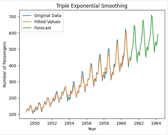 Visualizing Triple Exponential Smoothing
How to Choose an Exponential Smoothing Technique
The selection of an exponential smoothing method is dependent on the properties of the time series and the forecasting needs such as forecast horizon, desired accuracy and available historical data.
| Method | When to Use | Description | Example |
|---|
| Simple Exponential Smoothing (SES) | Time series with no trend or seasonality. | Uses the most recent data point to forecast. Applied when data is stationary without clear trend or seasonality. | Stock prices without a trend or season. |
|---|
| Holt’s Linear Smoothing | Time series with a trend but no seasonality. | Extends SES to account for a linear trend. Forecasts data with consistent upward or downward movement. | Sales data with steady growth. |
|---|
| Holt-Winter’s Seasonal Smoothing | Time series with both trend and seasonality. | Adds a seasonal component to the trend, capturing both. Used for time series with repeating patterns and trends. | Monthly temperature data or quarterly sales. |
|---|
It is important to test different methods and adjust smoothing parameters (like alpha and beta) to find the best approach for our data and forecasting needs.
Note: Always validate the forecast using out-of-sample data and evaluate accuracy with performance metrics before finalizing the model.
Advantages of Using Exponential Smoothing:
- Analysts can adjust the weighting of recent observations by modifying smoothing parameters (alpha, beta, etc.) making it adaptable to various forecasting needs.
- Unlike moving averages which assign equal weight to all data within the window, exponential smoothing gives more weight to recent data and models error, trend and seasonality.
- Exponential Smoothing models are referred to as ETS (Error, Trend, Seasonality) models similar to the Box-Jenkins ARIMA approach.
Limitations of Exponential Smoothing:
- May not perform well for time series with complex patterns such as sudden level or trend changes, outliers or abrupt seasonality.
- The accuracy of forecasts depends on the selection of smoothing parameters (alpha, beta, gamma) which may require trial and error or model selection techniques.
Explore
Introduction to AI
AI Concepts
Machine Learning in AI
Robotics and AI
Generative AI
AI Practice