Forward State Space Planning (FSSP) in AI
Last Updated :
21 Aug, 2025
Forward State Space Planning (FSSP) is an important technique in artificial intelligence (AI) that helps systems find how to reach a specific goal by taking a series of actions. This method involves exploring different possible states starting from an initial configuration and applying valid actions to transition through various states until the goal is achieved. It allows an AI to plan the most efficient sequence of actions to move from one state to another in order to meet its desired objective.
Key Concepts in FSSP
- Initial State: The starting point of the system, representing its current condition. For example, it could be the robot's position or the arrangement of objects in the environment.
- Actions: These are the steps the system can take to change its state. Each action has a specific effect and a precondition such as moving a robot in a particular direction or changing the environment.
- State Exploration: It explores all possible states the system can transition into by applying different actions. It works by evaluating each step to move closer to the goal.
- Goal State: The target state or condition that the system is trying to achieve. The process continues until the system reaches this goal.
FSSP is called progressive planning because it works by moving forward from the initial state step-by-step toward the goal.
Working of Forward State Space Planning
Forward State Space Planning (FSSP) works by systematically searching through the possible states to reach a goal from an initial state. Let’s see how it works step-by-steps:
- Starting Point (Initial State): It begins at the starting state, representing the initial configuration of the system.
- Action Selection: From the current state, it identifies all possible actions that can be taken. These actions are evaluated to find which ones move the system closer to the goal.
- State Transitions: Each selected action is applied, changing the state of the system. The new state is then treated as the current state for the next iteration.
- Exploration and Evaluation: It checks each new state and continues to evaluate possible actions from that state. It keeps track of the states already explored to avoid unnecessary repetition.
- Reaching the Goal: This process repeats until the goal state is found, at which point the planning process is complete.
Types of Search in FSSP
There are a few different search methods that can be used in FSSP, most common methods are:
- Breadth-First Search (BFS): This method explores all possible states level by level. It’s simple and guarantees the shortest path but can be slow if the state space is large.
- Depth-First Search (DFS): This method explores one path as deeply as possible before backtracking. It’s faster but it might miss the shortest path to the goal.
- A* Search: This method combines the benefits of BFS and DFS. It uses heuristics to prioritize states that are more likely to lead to the goal, making the search more efficient.
Forward State Space Planning with Breadth-First Search
Let’s see an example of how Forward State Space Planning (FSSP) can be implemented using the Breadth-First Search (BFS) algorithm. Here we’ll solve the problem of finding the shortest path in a grid-based environment with no obstacles.
Problem Setup:
- The environment is a grid where the agent can move in four directions: up, down, left and right.
- The task is to find the shortest path from a start position to a goal position.
Step 1: Importing the Required Libraries
We will be importing Matplotlib and Numpy libraries.
Python
import matplotlib.pyplot as plt
import numpy as np
from collections import deque
Step 2: Implementing Forward State Space Planning (FSSP) Class
Here we defines the FSSP_BFS class which implements Forward State Space Planning using the BFS algorithm. It initializes the grid, start position, goal position and the grid dimensions (rows and columns).
Python
MOVES = [(-1, 0), (1, 0), (0, -1), (0, 1)]

class FSSP_BFS:
    def __init__(self, grid, start, goal):
        self.grid = grid
        self.start = start
        self.goal = goal
        self.rows = len(grid)
        self.cols = len(grid[0])
Step 3: Checking for Valid Moves
The is_valid method checks if a given position is within the bounds of the grid and is not blocked represented by 1. This ensures that the agent only moves to valid positions.
Python
    def is_valid(self, position):
        r, c = position
        return 0 <= r < self.rows and 0 <= c < self.cols and self.grid[r][c] == 0
Step 4: Implementing BFS Algorithm for Pathfinding
The bfs method implements the Breadth-First Search algorithm to explore the grid. It starts from the initial position, explores valid neighboring positions (up, down, left, right) and keeps track of the path taken. Once the goal is reached, the method returns the path.
Python
    def bfs(self):
        queue = deque([(self.start, [self.start])])
        visited = set([self.start])

        while queue:
            current, path = queue.popleft()

            if current == self.goal:
                return path

            for move in MOVES:
                next_r, next_c = current[0] + move[0], current[1] + move[1]
                next_position = (next_r, next_c)

                if self.is_valid(next_position) and next_position not in visited:
                    visited.add(next_position)
                    queue.append((next_position, path + [next_position]))

        return None
Step 5: Visualizing the Grid and Path
This method visualizes the grid and the path found by the BFS algorithm. It uses matplotlib to display the grid, marks the start (S) and goal (G) and highlights the path using blue lines with yellow markers. It also adds grid lines for better clarity.
Python
    def visualize(self, path):
        grid_np = np.array(self.grid)

        fig, ax = plt.subplots(figsize=(8, 8))
        ax.imshow(grid_np, cmap='Greys', alpha=0.8)

        ax.text(self.start[1], self.start[0], 'S', color='green', fontsize=18, fontweight='bold', ha='center', va='center')
        ax.text(self.goal[1], self.goal[0], 'G', color='red', fontsize=18, fontweight='bold', ha='center', va='center')

        if path:
            path_np = np.array(path)
            ax.plot(path_np[:, 1], path_np[:, 0], color='blue', linewidth=2.5, marker='o', markersize=10, markerfacecolor='yellow', label='Path')

        ax.set_xticks(np.arange(self.cols))
        ax.set_yticks(np.arange(self.rows))
        ax.set_xticklabels(np.arange(self.cols))
        ax.set_yticklabels(np.arange(self.rows))
        ax.grid(which='both', color='black', linewidth=1.5)

        plt.title("Enhanced Grid and Path Visualization", fontsize=16, fontweight='bold')
        plt.tight_layout()
        plt.show()
Step 6: Defining the Grid and Setting Up the Planner
Here we sets up the grid, start position and goal position. It initializes the FSSP_BFS planner, calls the BFS algorithm to find the path and then visualizes the result. If no path is found, it outputs "No path found."
Python
grid = [
    [0, 0, 0, 1, 0],
    [0, 1, 0, 1, 0],
    [0, 1, 0, 0, 0],
    [0, 0, 0, 1, 0],
    [1, 1, 0, 0, 0]
]
start = (0, 0)
goal = (4, 4)

planner = FSSP_BFS(grid, start, goal)
path = planner.bfs()

if path:
    print(f"Path found: {path}")
    planner.visualize(path)
else:
    print("No path found")
Output:
Path found: [(0, 0), (1, 0), (2, 0), (3, 0), (3, 1), (3, 2), (4, 2), (4, 3), (4, 4)]
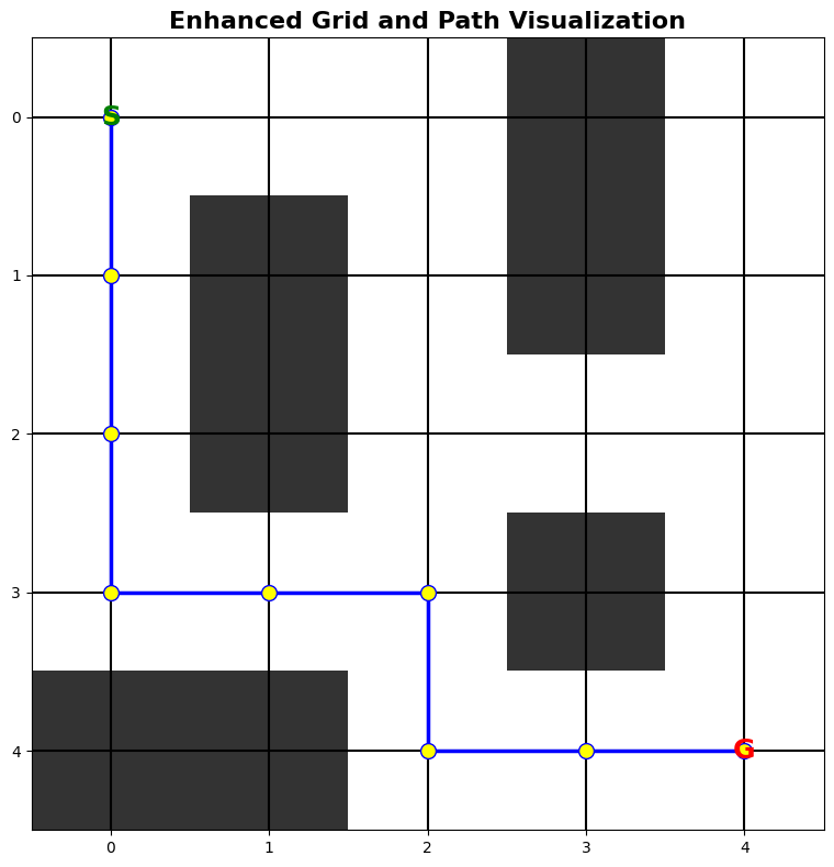 Path Visualization
Enhancing FSSP Efficiency
To improve scalability and efficiency in Forward State Space Planning (FSSP), AI researchers have developed key techniques:
- Heuristic Search: Heuristic techniques guide the search process by estimating how close a state is to the goal, enabling the algorithm to focus on more promising paths. Algorithms like A* use heuristics to prioritize states that are likely to lead to the goal faster, optimizing the search by reducing unnecessary exploration of less relevant states.
- Pruning: Pruning techniques such as alpha-beta pruning and branch-and-bound help reduce the search space by cutting off branches that are unlikely to provide better solutions. By eliminating states or paths that have already been explored or have no potential for improvement, pruning increases the efficiency of the search process and speeds up problem-solving in large-scale state spaces.
Applications of FSSP
FSSP has been applied in several AI domains including:
- Robotics: In autonomous robotics, it can be used for path planning and navigation tasks. Robots can use FSSP to decide which sequence of movements will lead them from an initial position to a target destination.
- Game Playing: In AI for games like puzzle-solving and strategic games like chess or Go, it can be used to explore all possible moves and predict the outcome of each one to find the optimal strategy.
- Logistics and Scheduling: It is applied in logistics for tasks such as route planning and resource scheduling. In this context, actions might include transporting goods or assigning workers to tasks in a way that optimizes for efficiency or cost.
- Automated Planning and Problem Solving: It is used to plan sequences of actions that enable the system to achieve specific mission objectives such as landing on a planet or driving in a complex urban environment.
Advantages of FSSP
- Deterministic and Predictable: It operates in environments where outcomes of actions are predictable, ensuring a straightforward and efficient planning process.
- Systematic Exploration: It explores the entire state space considering all possible actions, making it reliable for finding the optimal solution.
- Easily Implemented with Classical Search Algorithms: It works well with well-established search algorithms like BFS and A*, making it easy to implement and integrate into existing systems.
Limitations of FSSP
While FSSP is effective, it has some limitations:
- Scalability Issues: As the problem grows in size, the state space (the number of possible states and transitions) can grow quickly. This makes searching through all possible states computationally expensive.
- Complexity of Actions: Some actions have complex conditions, making it difficult to predict the outcomes and manage state transitions.
- Resource Constraints: AI systems have limited computational resources so searching through a large state space may not be practical.
Explore
Introduction to AI
AI Concepts
Machine Learning in AI
Robotics and AI
Generative AI
AI Practice