Uniform Cost Search (UCS) in AI

Uniform Cost Search (UCS) is a search algorithm used in artificial intelligence (AI) for finding the least cost path in a graph. It is a variant of Dijkstra's algorithm and is particularly useful when all edges of the graph have different weights, and the goal is to find the path with the minimum total cost from a start node to a goal node. In this article, we will explore the fundamentals of UCS, its working mechanism, and its applications in AI.

Introduction to Uniform Cost Search (UCS)

Uniform Cost Search is a pathfinding algorithm that expands the least cost node first, ensuring that the path to the goal node has the minimum cost. Unlike other search algorithms like Breadth-First Search (BFS), UCS takes into account the cost of each path, making it suitable for weighted graphs where each edge has a different cost.

Key Concepts of Uniform Cost Search

1. Priority Queue: UCS uses a priority queue to store nodes. The node with the lowest cumulative cost is expanded first. This ensures that the search explores the most promising paths first.
2. Path Cost: The cost associated with reaching a particular node from the start node. UCS calculates the cumulative cost from the start node to the current node and prioritizes nodes with lower costs.
3. Exploration: UCS explores nodes by expanding the least costly node first, continuing this process until the goal node is reached. The path to the goal node is guaranteed to be the least costly one.
4. Termination: The algorithm terminates when the goal node is expanded, ensuring that the first time the goal node is reached, the path is the optimal one.

Working Uniform Cost Search

UCS operates under a simple principle: among all possible expansions, pick the path that has the smallest total cost from the start node. This is implemented using a priority queue to keep the partial paths in order, based on the total cost from the root node.

Here’s the step-by-step process of how UCS works:

1. Initialization: UCS starts with the root node. It is added to the priority queue with a cumulative cost of zero since no steps have been taken yet.
2. Node Expansion: The node with the lowest path cost is removed from the priority queue. This node is then expanded, and its neighbors are explored.
3. Exploring Neighbors: For each neighbor of the expanded node, the algorithm calculates the total cost from the start node to the neighbor through the current node. If a neighbor node is not in the priority queue, it is added to the queue with the calculated cost. If the neighbor is already in the queue but a lower cost path to this neighbor is found, the cost is updated in the queue.
4. Goal Check: After expanding a node, the algorithm checks if it has reached the goal node. If the goal is reached, the algorithm returns the total cost to reach this node and the path taken.
5. Repetition: This process repeats until the priority queue is empty or the goal is reached.

Implementing Uniform Cost Search to Solve Pathfinding Problem

Step 1: Import Required Libraries

This step imports the necessary libraries for implementing Uniform Cost Search (UCS) and visualizing the graph.

import heapq
import networkx as nx
import matplotlib.pyplot as plt

Step 2: Define the Uniform Cost Search Function

This function implements the UCS algorithm to find the least cost path from a start node to a goal node in a weighted graph.

def uniform_cost_search(graph, start, goal):
    
    priority_queue = [(0, start)]
    # Dictionary to store the cost of the shortest path to each node
    visited = {start: (0, None)}
    
    while priority_queue:
        # Pop the node with the lowest cost from the priority queue
        current_cost, current_node = heapq.heappop(priority_queue)
        
        # If we reached the goal, return the total cost and the path
        if current_node == goal:
            return current_cost, reconstruct_path(visited, start, goal)
        
        # Explore the neighbors
        for neighbor, cost in graph[current_node]:
            total_cost = current_cost + cost
            # Check if this path to the neighbor is better than any previously found
            if neighbor not in visited or total_cost < visited[neighbor][0]:
                visited[neighbor] = (total_cost, current_node)
                heapq.heappush(priority_queue, (total_cost, neighbor))
    
    return None

Step 3: Define the Path Reconstruction Function

This function reconstructs the path from the start node to the goal node by tracing back through the visited nodes.

def reconstruct_path(visited, start, goal):
    # Reconstruct the path from start to goal by following the visited nodes
    path = []
    current = goal
    while current is not None:
        path.append(current)
        current = visited[current][1]  # Get the parent node
    path.reverse()
    return path

Step 4: Define the Visualization Function

This function visualizes the graph and the path found by UCS, using networkx for graph creation and matplotlib for visualization.

def visualize_graph(graph, path=None):
    G = nx.DiGraph()

    # Adding nodes and edges to the graph
    for node, edges in graph.items():
        for neighbor, cost in edges:
            G.add_edge(node, neighbor, weight=cost)

    pos = nx.spring_layout(G)  # Positioning the nodes

    # Drawing the graph
    plt.figure(figsize=(8, 6))
    nx.draw(G, pos, with_labels=True, node_color='lightblue', node_size=2000, font_size=15, font_weight='bold', edge_color='gray')
    labels = nx.get_edge_attributes(G, 'weight')
    nx.draw_networkx_edge_labels(G, pos, edge_labels=labels, font_size=12)

    if path:
        # Highlight the path in red
        path_edges = list(zip(path, path[1:]))
        nx.draw_networkx_edges(G, pos, edgelist=path_edges, edge_color='red', width=2.5)

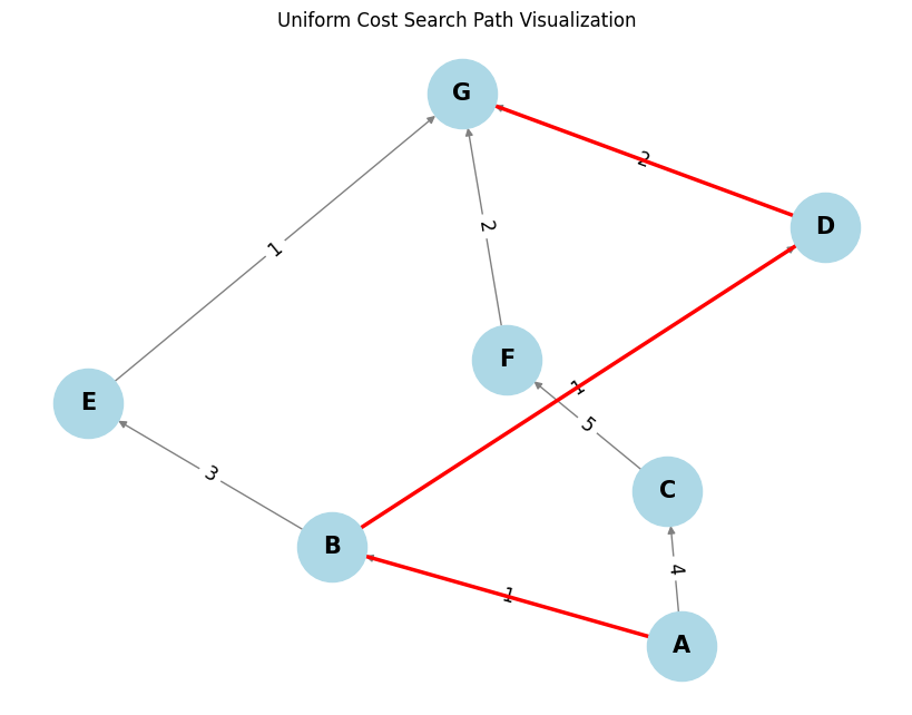
    plt.title("Uniform Cost Search Path Visualization")
    plt.show()

Step 5: Define the Graph and Execute UCS

This step defines a sample graph as an adjacency list, sets the start and goal nodes, and runs the UCS algorithm. It then visualizes the graph and the path found.

# Example graph represented as an adjacency list
graph = {
    'A': [('B', 1), ('C', 4)],
    'B': [('D', 1), ('E', 3)],
    'C': [('F', 5)],
    'D': [('G', 2)],
    'E': [('G', 1)],
    'F': [('G', 2)],
    'G': []
}

# Example usage of the UCS function
start_node = 'A'
goal_node = 'G'
result = uniform_cost_search(graph, start_node, goal_node)

if result:
    total_cost, path = result
    print(f"Least cost path from {start_node} to {goal_node}: {' -> '.join(path)} with total cost {total_cost}")
    visualize_graph(graph, path)
else:
    print(f"No path found from {start_node} to {goal_node}")

Output:

Least cost path from A to G: A -> B -> D -> G with total cost 4

You can download the complete code from here.

Applications of UCS in AI

Uniform Cost Search is widely applicable in various fields within AI:

1. Pathfinding in Maps: Determining the shortest route between two locations on a map, considering different costs for different paths.
2. Network Routing: Finding the least-cost route in a communication or data network.
3. Puzzle Solving: Solving puzzles where each move has a cost associated with it, such as the sliding tiles puzzle.
4. Resource Allocation: Tasks that involve distributing resources efficiently, where costs are associated with different allocation strategies.

Advantages of Uniform Cost Search

• Optimality: UCS is guaranteed to find the least cost path to the goal state if the cost of each step exceeds zero.
• Completeness: This algorithm is complete; it will find a solution if one exists.

Challenges with UCS

• Space Complexity: The main drawback of UCS is its space complexity. The priority queue can grow significantly, especially if many nodes are being expanded.
• Time Complexity: The time it takes to find the least cost path can be considerable, especially if the state space is large.