Navigating large datasets in Excel can quickly become overwhelming, especially when key headers or reference columns disappear as you scroll. That’s where the freeze panes feature comes in. Freeze panes in Excel allow you to lock specific rows or columns in place, ensuring critical data remains visible while you work. Whether you’re dealing with complex spreadsheets or simply trying to keep your headers accessible, this tool is a game-changer for improving Excel data management tools and navigation efficiency.
Disclaimer: Double-check your data and settings before applying changes to avoid losing critical information.
What is the Freeze Panes Feature in Excel
Freeze Panes is a feature in Excel that allows you to lock specific rows or columns in place so they remain visible while you scroll through the rest of the worksheet. This is particularly useful when working with large datasets, as it helps you keep important headers, labels, or identifiers in view while analyzing the data below or to the side.
Key Features of Freeze Panes
- Freezing the Top Row: Keeps the first row visible, usually used for column headers.
- Freezing the First Column: Locks the first column in place, often used for row labels or identifiers.
- Custom Freeze Panes: Allows you to freeze multiple rows and/or columns based on your selection.
This feature is essential for improving navigation and readability, especially in complex spreadsheets where data spans across many rows and columns
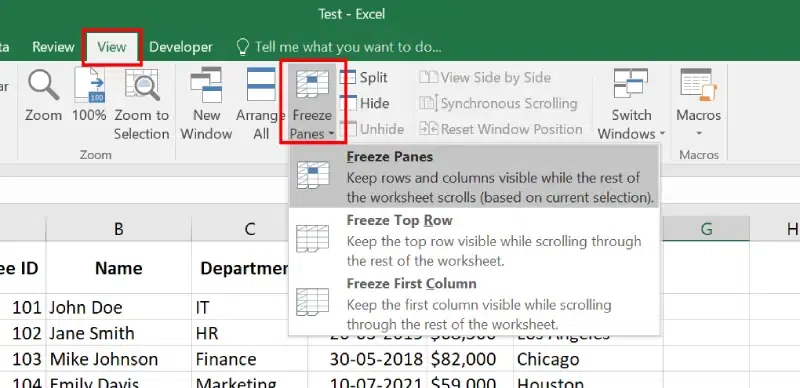
 View Tab>> Freeze Panes in Excel
How to Freeze Rows in Excel
Freezing rows in Excel helps you lock rows in Excel so they remain visible while scrolling through your data. Follow this freeze panes Excel step-by-step guide:
Step 1: Open your Excel Sheet
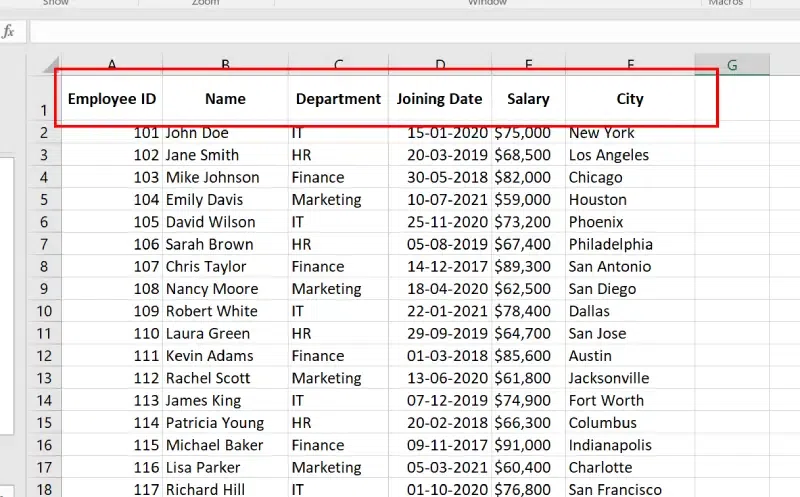
Open the Excel sheet where you want to freeze the top row. Ensure that the first row of your worksheet contains the headers or labels you want to keep visible. For example, in the dataset below, the top row contains headers such as Employee ID, Name, Department, Joining Date, Salary, and City, which we aim to freeze.
 Header Row
Step 2: Use the Freeze Panes Option
Click on the View tab located in the Ribbon, Select the Freeze Panes Dropdown, and Select Freeze Top Row from the dropdown menu.
Use can also use Freeze Panes Shortcuts
- For Windows: Press
Alt + W + F + R. - For Mac: Press
Cmd + Option + R.
 Go to View Tab>> Select Freeze Panes >> Freeze Top Row
Step 3: Preview Result
Scroll down your worksheet to confirm that the top row remains fixed while the other rows move. A faint horizontal line will appear below the frozen row, indicating that it’s locked.
 Preview Results
How to Freeze Column in Excel
Freezing the first column in Excel helps keep the column visible while scrolling horizontally through your data. This is particularly useful when the first column contains identifiers like names, IDs, or labels that you need to reference while reviewing other data. Follow the below steps to know how to freeze column in excel:
Step 1: Open Excel Spreadsheet
Open the Excel file where you want to freeze the first column. Ensure it contains key data or labels like employee names or product IDs. In the example below, the first column contains Employee IDs.
 Open Excel Spreadsheet
Step 2: Use the Freeze Panes Option
Click on the View tab located in the Ribbon, Select the Freeze Panes Dropdown, and Select Freeze First Column from the dropdown menu. This action will lock the first column, ensuring it remains visible as you scroll horizontally across the worksheet.
You can also Use Shortcut to Freeze First Column
- For Windows: Press
Alt + W + F + C. - For Mac: Press
Cmd + Option + C.
 View Tab>>Freeze Panes>>Freeze First Column
Note: Freezing First Column and Top Row only freezes the one row/column to the screen. To freeze multiple, the Freeze Panes option is used.
Step 3: Verify the Results
You’ll notice a thin gray line to the right of the first column, indicating that the column is now frozen. Scroll horizontally through your data to confirm that the first column remains in view.
 Preview Results
How to Freeze Multiple Rows in Excel
Freezing multiple rows in Excel is useful when working with large datasets where you want to keep specific rows always visible while scrolling through the rest of the sheet. Here’s a step-by-step guide:
Step 1: Open Your Excel File
Open the Excel file where you want to freeze multiple rows. Ensure the rows you want to freeze contain important headers or information you need to keep visible.
Step 2: Select the row below the rows to freeze.
Click on the row number directly below the last row you want to freeze. For example, if you want to freeze rows 1 to 3, select row 4 by clicking its number on the left.
Step 3: Use the Freeze Panes Option
Navigate to the View tab in the Ribbon and click the Freeze Panes dropdown. From the menu, select Freeze Panes to lock all rows above the selected row, keeping them visible as you scroll through the worksheet.
Shortcut:
Select the cell below the rows (and to the right of the columns, if needed) you want to freeze.
- For Windows: Press
Alt + W + F + F. - For Mac: Manually go to View > Freeze Panes.
 Go to View Tab>> Freeze Panes Dropdown>> Select Freeze Panes
Step 4: Preview Result
Scroll down in your worksheet to confirm that the rows above the selected row remain visible. The freeze line will appear below the last frozen row.
 Preview Result
How to Freeze Multiple Columns in Excel
Freezing multiple columns in Excel helps keep important data visible as you scroll horizontally through your worksheet. Follow these steps to freeze multiple columns:
Step 1: Open Your Worksheet
Open the Excel file where you want to freeze multiple columns. Ensure the columns you want to freeze are positioned on the left side of the worksheet.
Step 2: Select the Column After the Last Column to Freeze
Click on the header of the column immediately to the right of the last column you want to freeze.
For example: If you want to freeze columns A and B, select column C.
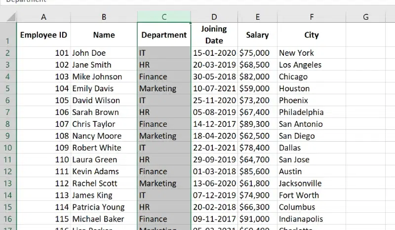
 Select a Row
Step 3: Use Freeze Panes
Go to the View tab in the Ribbon at the top of the screen and click on the Freeze Panes dropdown menu. Once you select Freeze Panes, scroll horizontally through your worksheet to confirm that the frozen columns (e.g., A and B) remain visible, making data navigation easier.
Shortcut to Freeze Multiple Rows/Columns
Select the cell below the rows and to the right of the columns you want to freeze.
- Windows:
Alt + W + F + F - Mac: Go to View > Freeze Panes manually.
 Select Column>> View Tab>> Freeze Panes Drop Down>>Freeze Panes
Step 4: Preview Results
After selecting Freeze Panes, scroll horizontally through your worksheet. The columns you froze (e.g., A and B) will remain visible, ensuring easier navigation of your data.
 Preview Results
How to Unfreeze Panes in Excel
When working with Excel, you may need to unfreeze panes to restore the default scrolling behavior. Unfreezing panes removes any locked rows or columns, allowing your entire worksheet to scroll freely.
Step 1: Open the Excel File
Open the Excel file where panes have been frozen. Ensure that the worksheet with frozen rows or columns is active. Here Row 1, 2 and 3 are frozen.
 Row 1,2 and 3 are Frozen
Step 2: Unfreeze Panes
In the Ribbon at the top of the screen, go to the View tab. Click on the Freeze Panes dropdown menu, and select Unfreeze Panes from the options. This will unfreeze any rows or columns that were previously locked, allowing you to scroll freely through your worksheet.
 View>>Freeze Panes Drop Down>>Unfreeze Panes
Step 3: Preview Results
After selecting Unfreeze Panes, scroll through the worksheet to confirm that the locked rows or columns are no longer frozen and the entire sheet scrolls freely.
 Preview Results
Notes:
- If Unfreeze Panes is grayed out, it means there are no frozen panes in the current worksheet.
- Unfreezing panes does not affect your data or formatting—it simply removes the freeze view.
Explore
Excel Fundamental
Excel Formatting
Excel Formula & Function
Excel Data Analysis & Visualization
Advanced Excel
Excel Data Visualization
Excel VBA & Macros
Power BI & Advance Features in Excel