How to Use HLOOKUP in Excel (Formula & Examples)
Last Updated :
03 Feb, 2025
Excel HLOOKUP Function - Quick Steps
- Select the cell
- Enter the HLOOKUP formula
- Input arguments>>Press Enter
Excel is packed with features that make handling and analyzing data easier. One of these handy tools is the HLOOKUP function, which is great for finding information in tables that are organized horizontally. The "H" in HLOOKUP stands for "horizontal," meaning it looks across the top row of a table to find a value, and then retrieves data from a specific row underneath. Whether you're working with a wide table or need to quickly find data in specific rows, HLOOKUP can help make your tasks faster and more efficient.
In this article, you will learn how to use the HLOOKUP Function in Excel, understand its HLOOKUP syntax, and explore practical HLOOKUP examples in Excel like working with multiple worksheets or even different workbooks.
Try using the new XLOOKUP function, An improved version of HLOOKUP that works in any direction and gives the exact match by default.
 Excel HLOOKUP Function with Formula and Examples
What is the HLOOKUP Function in Excel
The HLOOKUP Function in Excel searches for a value in the top row of a table or array and returns a value in the same column from a specified row. Although less popular than its vertical counterpart, VLOOKUP, this function is ideal for data arranged horizontally, where lookup values are stored in the first row.
When to Use the HLOOKUP Function in Excel
The HLOOKUP Function is most useful when:
- Your data is organized horizontally.
- You need to retrieve information from a specific row based on a lookup value.
- You require exact or approximate matches in your lookup operation.
HLOOKUP Syntax & Parameters
The syntax of the HLOOKUP function is as follows:
HLOOKUP(lookup_value, table_array, row_index_num, [range_lookup])
Where:
- lookup_value: The value you want to search for in the top row of the table.
- table_array: The range of cells that contains the data. The top row of this range will be searched for the lookup_value.
- row_index_num: The row number in the table_array from which to return a value. The top row is row 1.
- [range_lookup]: An optional argument. Use TRUE for an approximate match (default), or FALSE for an exact match.
How to Use HLOOKUP Formula in Excel
The HLOOKUP formula is a useful tool for looking up data in tables arranged horizontally. This HLOOKUP tutorial will guide you through the steps to use the function effectively:
Step 1: Prepare your Data
Organize your data so that the lookup value resides in the first row of a range or table. For Example:
 Prepare your Data
Select a blank cell where you want the result of the HLOOKUP function to appear. In the below example we have selected B5.
 Select a Cell where you want to display the results
To look up the sales for Q3, enter the following formula in your selected cell:
=HLOOKUP("Q3", A1:E2, 2, FALSE)Step 4: Press Enter
After pressing Enter, Excel will return 2500, which is the value in the second row under "Q3."
 Select the Cell>> Enter the Formula>> Press Enter
Excel HLOOKUP Function with Formula Examples
The HLOOKUP function is a powerful tool in Excel that helps you find data arranged horizontally in a table. In this section, you’ll explore HLOOKUP examples in Excel that demonstrate how to use the function for quick and efficient data retrieval.
Example 1: Finding an Exact Match
Suppose you have a grade table where the first row contains scores and the second row contains grades.
 Prepare your Data
To find the grade for a score of 80, use the formula:
=HLOOKUP(80, A1:F2, 2, FALSE)
Result: Excel will return B.
 Excel will return B.
Example 2: Approximate Match in HLOOKUP
For approximate matches, set the range_lookup argument to TRUE.
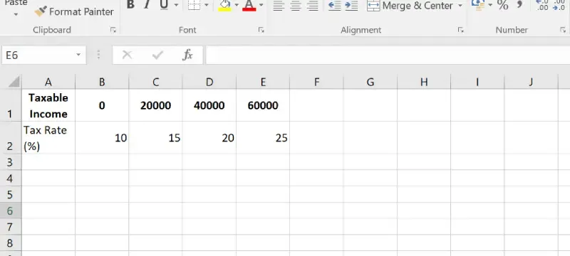 Approximate Match
To find the tax rate for an income of 45000, use the formula:
=HLOOKUP(45000, A1:E2, 2, TRUE)
Result: Excel will return 20, as 45000 is between 40000 and 60000.
 Enter the data >> Use the Formula
Example 3: Using Wildcards with HLOOKUP
Using Asterisk (*) for Partial Matches. You want to find the quantity of any category that starts with "F" (e.g., "Fruits").
 HLOOKUP With Wildcards
Formula:
=HLOOKUP("F*",A1:D2,2,FALSE)Result: 50 (The quantity for "Fruits").
 Use the Formula
How to Use HLOOKUP Across Two Worksheet
Using the HLOOKUP formula across two worksheets in Excel is a great way to retrieve data from one sheet while working on another. This can be especially helpful when managing large datasets spread over multiple sheets.
Let's Suppose you have two worksheets: Sheet1 and Sheet2. To extract our matching data from another worksheet, mention the sheet name followed by an exclamation mark.
Step 1: Identify the Lookup Value
In Sheet1, locate the cell containing the lookup value (e.g., B1) that you want to search for in Sheet2.
 Identify the Lookup Value
Step 2: Specify the Data Range in the Other Sheet
- Reference Sheet2 in your formula by including the sheet name followed by an exclamation mark (
!). - Example data range in Sheet2:
A1:F2.
- In Sheet1, input the following formula to perform the lookup
=HLOOKUP(B1, Sheet2!A1:F2, 2, FALSE)
B1: The lookup value in Sheet1.Sheet2!A1:F2: The data range in Sheet2 containing the lookup table.2: Specifies the row number in the lookup table from which to retrieve the result.FALSE: Ensures an exact match.
Drag the formula down or across other cells in Sheet1 to copy the HLOOKUP formula, dynamically referencing the lookup values.
 Drag the Formula
Data from sheet 2 (sold) is copied from sheet 2 to sheet 1.
How to Use HLOOKUP with Another Workbook
The HLOOKUP function in Excel becomes even more powerful when you use it to retrieve data across multiple workbooks. This can help you manage large datasets stored in different files without the need to combine them manually.
Suppose you have two workbooks: Workbook1.xlsx and Workbook2.xlsx. You want to retrieve data from Book2.xlsx into Book1.xlsx.
Step 1: Open Both Workbooks
Ensure both workbooks are open in Excel.
 Enter data in two different workbooks
Step 2: Reference the External Workbook
In Book1.xlsx, write the formula referencing Book2.xlsx. The external workbook name should be enclosed in square brackets ([]) and followed by the sheet name and range.
For example, to retrieve data from Sheet1 of Book2.xlsx, use the following formula:
=HLOOKUP(A2, [Workbook2.xlsx]Sheet1!A1:F2, 2, FALSE)
 Enter the Formula in Book1
If the external workbook is closed, the file path will be automatically included in the formula.
For Example:
=HLOOKUP(A2, 'C:\Documents\[Workbook2.xlsx]Sheet1'!A1:F2, 2, FALSE)
Copy or drag the formula to other cells as needed to reference corresponding lookup values.
 Copy down the Formula
This setup shows how HLOOKUP works between two workbooks, retrieving data dynamically from the Sales row in Book2.xlsx into Book1.xlsx.
Things to Keep in Mind When Using HLOOKUP
- The lookup_value must always be in the top row of the table_array.
- The table_array should contain multiple rows and columns for HLOOKUP to work.
- HLOOKUP is case-insensitive, so "jane" and "Jane" will be treated as the same.
- If HLOOKUP cannot find the lookup_value, it will return an #N/A error.
- For approximate matches, the table_array should be sorted in ascending order.
Difference Between VLOOKUP and HLOOKUP
VLOOKUP and HLOOKUP are both lookup functions in Excel, but they work differently based on how your data is organized.
| Feature | VLOOKUP | HLOOKUP |
|---|
| Orientation | Searches data vertically (in columns). | Searches data horizontally (in rows). |
| Search Direction | Finds a value in the first column and retrieves from a specified row. | Finds a value in the first row and retrieves from a specified column. |
| Best Use | Use when data is organized in columns. | Use when data is organized in rows. |
Limitations of HLOOKUP
- HLOOKUP can only search for the lookup_value in the top row and return values from rows below it. If your data is not organized this way, you may need to rearrange your data or use other functions like INDEX and MATCH.
- Unlike VLOOKUP, you cannot look to the left of the lookup_value; it can only return values from rows below the lookup_value row.
Conclusion
The HLOOKUP function is a valuable tool in Excel when you need to search for data across horizontal rows. Whether you're working with monthly sales data, grades, or employee information, HLOOKUP makes it easier to retrieve specific values based on a reference from the top row.
By understanding the HLOOKUP formula, applying the correct row_index_num, and deciding between exact and approximate matches, you can efficiently perform horizontal lookups to analyze your data and make informed decisions.
Similar Reads
Excel SUMIF Function: Formula, How to Use and Examples
The SUMIF function in Excel is a versatile tool that enables you to sum values based on specific criteria, such as a true or false condition. This feature makes it perfect for conditional summation tasks like totaling sales over a particular amount, adding up expenses in specific categories, or summ
7 min read
How to Decide Which Excel Lookup Formula to Use?
In Excel, you have a ton of methods to look upon the specific types of values, but the optimal method chosen is what creates a difference. So, what mindset we need to use specific lookup methods in a situation? That's what we will look at here. But, first, let's take a look at an example from real l
15 min read
How To Use MATCH Function in Excel (With Examples)
Finding the right data in large spreadsheets can often feel like searching for a needle in a haystack. This is where the MATCH function in Excel proves invaluable. The MATCH function helps you locate the position of a specific value within a row or column, making it a cornerstone of efficient data m
6 min read
How to Create a Formula in Excel using Java?
Apache POI is a popular open-source Java library that provides programmers with APIs for creating, modifying, and editing MS Office files. Excel is very excellent at calculating formulas. And perhaps most Excel documents have formulas embedded. Therefore, it’s trivial that on a fine day, you have to
3 min read
How to Combine Excel Functions in a Formula?
We all use Excel for some small computations in data but excel also provides the functionality to combine these small functions and make a formula for manipulating the data. For example, let's say that in school we need to increment the ID numbers of students by a number but the ID's have some text
2 min read
How to Create an Array Formula in Excel?
Array formulas in excel are important tools. A single formula can perform multiple calculations and replace thousand of useful formulas. Most of us have never used array functions in our excel sheet just because we don't know how to use these formulas. Array formulas is one of the most confusing exc
10 min read
Excel Date Functions with Formula Examples
There are many functions in Microsoft Excel that may be used to work with dates and timings in Excel. Each function completes a straightforward task, but by combining numerous functions into a single formula, you may handle trickier and more complicated problems. The purpose of discussing DATE funct
12 min read
How to Use ChatGPT to Write Excel Formulas
Worrying about mastering Excel formulas? Thinking about the right syntax and function for hours? If you are, ChatGPT has got you covered! Discover how ChatGPT makes Excel formula writing effortless in the following article. In data analysis, Excel formulas reign supreme as a crucial tool. They make
5 min read
How to Use Flash Fill in Excel?
Excel Flash Fill is a highly time-saving tool that allows you to automatically fill in values. Flash Fill tries to detect the consistent pattern you type and show a faded list of suggestions. If you find the suggested list suitable, press Enter. It is highly used to split data from one column to dif
3 min read
How to use Conditional Formatting in Excel?
Microsoft Excel is a software that allows users to store or analyze the data in a proper systematic manner. It uses spreadsheets to organize numbers and data with formulas and functions. MS Excel has a collection of columns and rows that form a table. Generally, alphabetical letters are assigned to
4 min read