How to Lock Cells In Excel: A Complete Guide

How to Protect Cells in Excel Spreadsheet- Quick Steps

• Select the cells you want to protect.
• Right-click, choose Format Cells>>Go to the Protection tab>> check Locked.
• Go to the Review tab>> click Protect Sheet >> set a password (optional) >>click OK.

Locking cells in Excel or Protecting Cells in Spreadsheet is essential for protecting your data from unintended edits, especially in shared or collaborative workbooks. When you lock cells, you can prevent changes to specific parts of a worksheet, ensuring that formulas, values, and structure remain intact.

This complete guide covers everything you need to know about locking cells in Excel. From locking specific cells or formulas to protecting entire worksheets, we’ll walk you through step-by-step instructions. You’ll also learn how to lock cells without protecting the entire sheet, unlock cells when needed, and even freeze rows and columns for easier navigation.

Why Lock Cells in Excel

Locking cells in Excel is helpful when you want to:

• Protect formulas from accidental changes.
• Limit access to specific areas in a shared workbook.
• Ensure that certain values and structures remain consistent and untouched.
• Allow only authorized users to edit specific cells.

How to Lock Specific Cells in Excel

If you want to protect specific cells but allow edits to others, follow these steps:

Step 1: Select the Cells to Lock

Highlight the cells or range of cells you want to lock. 

Step 2: Right Click and Select Format Cells

Right-click the selected cells and choose Format Cells, or press Ctrl + 1 to open the Format Cells dialog box.

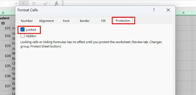
Step 3: Enable the Locked Option

• In the Format Cells dialog, go to the Protection tab and check the Locked option.
• Click OK to apply the changes.

Step 4: Protect the Worksheet

• Go to the Review tab in the Excel Ribbon.
• Click Protect Sheet
• If desired, enter a password to prevent unauthorized users from unprotecting the sheet.
• Click OK to apply the protection.

Step 5: Preview the Results

Excel will display a warning, as shown in the image below, if you attempt to make any changes to locked cells.

How to Lock All Cells in Excel

To lock all cells in an Excel worksheet, follow these steps:

Step 1: Select All Cells

Press Ctrl + A to select the entire worksheet.

Step 2: Open the Format Cells Dialog

Right-click on any selected cell and choose Format Cells.

Step 3: Enable the Locked Option

• Go to the Protection tab in the Format Cells dialog.
• Make sure the Locked checkbox is checked and click OK.

Step 4: Protect the Sheet

• Go to the Review tab and click Protect Sheet.

Step 5: Preview Results

Excel will show a warning alert if you attempt to edit the data in locked cells.

How to Protect a Worksheet in Excel

Protecting a worksheet in Excel not only locks cells but also ensures that your entire sheet (or specific parts of it) is safeguarded from unwanted changes. Here’s how you can protect a worksheet step by step:

Step 1: Go to the Review Tab

Navigate to the Review tab in the Excel toolbar (or press Alt + R)

Step 2: Click on "Protect Sheet"

In the Review tab, click Protect Sheet. A dialog box will appear.

Alternatively Press the Shortcut (Alt + R + P + S)

Step 3: Set a Password (Optional)

Enter a password if you want to restrict access to the protection settings. Make sure to remember this password, as it will be required to unprotect the sheet.

Step 4: Choose the Protection Options

Select which actions users can perform, such as:

• Selecting locked or unlocked cells
• Formatting cells
• Inserting rows or columns
• Deleting columns or rows

Step 5: Click OK

Confirm your settings by clicking OK.

Your worksheet is now protected, meaning any locked cells cannot be edited unless the sheet is unprotected. This is a great way to ensure the integrity of your data, especially when sharing your spreadsheet with others.

Tip: If you need to make changes later, you can unprotect the sheet by returning to the Review tab and clicking Unprotect Sheet. Enter the password if prompted.

How to Lock Formulas in Excel

To protect only the cells containing formulas while allowing other cells to remain editable, follow these steps:

Disclaimer: Always Unlock Non-Formula Cells First!

Before protecting the sheet, make sure to unlock non-formula cells if you want them to remain editable. Select those cells, go to Format Cells → Protection, and uncheck "Locked".

Step 1: Select All Cells

• Press Ctrl + A to select the entire worksheet.

Step 2: Unlock All Cells

• Right-click the selected cells and choose Format Cells (Ctrl + 1).
• In the Protection tab, uncheck the Locked box.
• Click OK to apply the changes.

Step 3: Select Formula Cells

• Go to the Home tab, click Find & Select, and choose Go To Special (Or Press Ctrl + G).
• Select Formulas and click OK to highlight all the cells that contain formulas.

Step 4: Lock Formula Cells

• Right-click the selected formula cells and choose Format Cells ( Or Press Ctrl + 1)
• In the Protection tab, check the Locked box and click OK.

Step 5: Protect the Sheet

• Go to the Review tab and click Protect Sheet.
• Optionally, set a password to restrict changes.
• Click OK to apply the protection.

(Alternatively, Press the Shortcut Alt + R + P + S)

Result: The formula cells are now locked and cannot be edited, while other cells in the worksheet remain editable.

Lock Cells Without Protecting the Entire Sheet

If you want to restrict cell editing in Excel without locking the whole sheet, you can lock specific cells while leaving others editable. Here's how to do it:

Step 1: Select the Cells You Want to Protect

Highlight the cells you wish to lock.

Step 2: Open the Format Cells Dialog

Right-click the selected cells and choose Format Cells (or use the shortcut Ctrl + 1)

Step 3: Enable the Locked Option

In the Protection tab, ensure the Locked checkbox is checked.

Step 4: Allow Edit Ranges

Go to the Review tab and click Allow Edit Ranges.

Alternatively Use the Shortcut (Alt + R + R).

Step 5: Define the Range

In the Allow Users to Edit Ranges dialog box, click New to define the range of cells you want to lock.

How to Unlock Cell Lock in Excel

By default, all cells are locked for editing in a spreadsheet, but it has no effect until you protect the worksheet. If you need to remove the lock from previously locked cells:

Step 1: Select All Cells

Press "Ctrl+A" on your keyboard to select all cells. (To select a whole range of sheets).

Step 2: Select Format cells

Right-click on the selected cells and select the FormatCells option from the dropdown.
 

Step 3: Choose the Protection Tab and Uncheck the Locked

A prompt box will open on your screen under the Protection tab uncheck the Locked option. (Alternatively, you can press Ctrl+1). Click on the OK button.

How to Freeze Cells, Rows, and Columns in Excel

Freezing panes helps keep headers or specific rows and columns visible while scrolling through large datasets. Follow these steps to freeze cells, rows, or columns in Excel:

Step 1: Select the Cell, Row, or Column to Freeze

• To freeze a row: Select the row below the one you want to keep visible.
• To freeze a column: Select the column to the right of the one you want to keep visible.
• To freeze both rows and columns: Click on the cell below the row and to the right of the column you want to freeze.

Step 2: Open the View Tab

• Go to the View tab in the Excel ribbon.

Step 3: Apply the Freeze Panes Option

• Click on Freeze Panes in the Window group.
• Choose one of the following options:
  • Freeze Panes: Locks selected rows and columns.
  • Freeze Top Row: Locks the first row of the sheet.
  • Freeze First Column: Locks the first column of the sheet.

Tips and Best Practices for Cell Lock in Excel Spreadsheet

• Prevent selection of locked cells: While protecting the sheet, uncheck "Select locked cells."
• Add a Lock Cell button: To the Quick Access Toolbar for easier access.
• Use different formatting: For locked cells to distinguish them from editable cells.
• Set a password: To further secure the protected sheet.

These tips not only show how to protect some cells in Excel but also how to protect selected cells in Excel for better data management.

Conclusion

Locking cells in Excel is a must-know skill for anyone sharing or collaborating on spreadsheets. By following this guide, you’ve learned how to lock specific cells, protect entire worksheets, and even lock formulas to prevent accidental changes. You’ve also discovered how to unlock cells when necessary and freeze rows or columns for better visibility.

Now that you know how to lock cells in Excel, you can confidently share your work without worrying about unwanted edits.

parthmadan3739

Follow

Improve

Article Tags :

• Excel
• Excel-basics
• ExcelGuide