Isomap - A Non-linear Dimensionality Reduction Technique
Last Updated :
10 Nov, 2025
Isomap (Isometric Mapping) is a non-linear dimensionality reduction method that reduces features while keeping the structure of the data intact. It works well when the data lies on a curved or complex surface.
- Handles non-linear datasets better than PCA
- Preserves true manifold-based distances
- Helps visualize high-dimensional patterns
- Useful for images, shapes and other curved data
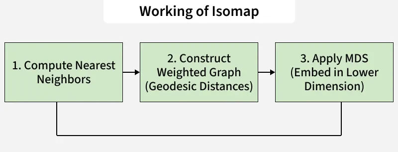 Working of Isomap
Manifold Learning
Manifold learning assumes that high-dimensional data actually lies on a lower-dimensional surface called a manifold. Example: A 2D sheet of paper twisted into a 3D spiral. Even though it appears 3D, its true structure is still 2D.
Manifold learning methods aim to unfold such shapes and find their simpler representation. In manifold learning we distinguish between two types of distances:
- Geodesic Distance is the shortest path between two points along the manifold’s surface
- Euclidean Distance is the straight-line distance between two points in the original space.
Isomap focuses on preserving geodesic distances because they show the true relationships in curved and non-linear datasets.
How Does Isomap Work?
Now that we understand the basics, let’s look at how Isomap works one step at a time.
- Calculate Pairwise Distances: First we find the Euclidean distances between all pairs of data points.
- Find Nearest Neighbors: For each point find the closest other points based on distance.
- Create a Neighborhood Graph: Connect each point to its nearest neighbors to form a graph.
- Calculate Geodesic Distances: Use algorithms like Floyd-Warshall to measure the shortest paths between points by following the graph connections.
- Perform Dimensional Reduction: Move points into a simpler space while keeping their distances as accurate as possible.
Implementation of Isomap with Scikit-learn
So far we have discussed about the introduction and working of Isomap, now lets understand its implementation to better understand it with the help of the visualization.
1. Applying Isomap to S-Curve Data
This part generates a 3D S-curve dataset and applies Isomap to reduce it to 2D for visualization. It highlights how Isomap preserves the non-linear structure by flattening the curve while keeping the relationships between points intact.
- make_s_curve() creates a 3D curved dataset shaped like an "S".
- Isomap() reduces the data to 2D while keeping its true structure.
Python
from sklearn.datasets import make_s_curve
from sklearn.manifold import Isomap
import matplotlib.pyplot as plt

X, color = make_s_curve(n_samples=1000, random_state=42)

isomap = Isomap(n_neighbors=10, n_components=2)
X_isomap = isomap.fit_transform(X)

fig, ax = plt.subplots(1, 2, figsize=(12, 5))

ax[0].scatter(X[:, 0], X[:, 2], c=color, cmap=plt.cm.Spectral)
ax[0].set_title('Original 3D Data')

ax[1].scatter(X_isomap[:, 0], X_isomap[:, 1], c=color, cmap=plt.cm.Spectral)
ax[1].set_title('Isomap Reduced 2D Data')

plt.show()
Output:
.jpg) Output of the above code
Output of the above codeScatter plot shows how Isomap clusters S shaped dataset together while preserving the dataset’s inherent structure.
2. Applying Isomap to Digits Dataset
Here Isomap is applied to the handwritten digits dataset that has 64 features per sample and reduces it to 2D. The scatter plot visually shows how Isomap groups similar digits together making patterns and clusters easier to identify in lower dimensions.
Python
from sklearn.datasets import load_digits
from sklearn.manifold import Isomap
import matplotlib.pyplot as plt

digits = load_digits()

isomap = Isomap(n_neighbors=30, n_components=2)
digits_isomap = isomap.fit_transform(digits.data)

fig, ax = plt.subplots(1, 2, figsize=(12, 5))

ax[0].scatter(digits.data[:, 0], digits.data[:, 1], c=digits.target, cmap=plt.cm.tab10)
ax[0].set_title('Original 2D Data (First Two Features)')

ax[1].scatter(digits_isomap[:, 0], digits_isomap[:, 1], c=digits.target, cmap=plt.cm.tab10)
ax[1].set_title('Isomap Reduced 2D Data')

plt.show()
Output:
.jpg) Output of the above code
Output of the above codeThe scatter plot shows how Isomap clusters similar digits together in the 2D space, preserving the dataset’s inherent structure.
Applications of Isomap
- Visualization: It makes it easier to see complex data like face images by turning it into 2D or 3D form so we can understand it better with plots or graphs.
- Data Exploration: It helps to find groups or patterns in the data that might be hidden when the data has too many features or dimensions.
- Anomaly Detection: Outliers or anomalies in the data can be identified by understanding how they deviate from the manifold.
- Pre-processing for Machine Learning: It can be used as a pre-processing step before applying other machine learning techniques improve model performance
Advantages of Isomap
- Captures Non-Linear Relationships: Unlike PCA Isomap can find complex, non-linear patterns in data.
- Preserves Global Structure: It retains the overall geometry of the data and provide a more accurate representation of the data relationships.
- Global Optimal Solution: It guarantees that the optimal solution is found for the neighborhood graph and ensure accurate dimensionality reduction.
Limitations of Isomap
- High Computation Time: Computing geodesic distances and shortest paths becomes slow when the dataset is large.
- Parameter Sensitivity: Results vary a lot if parameters like number of neighbors are not chosen properly.
- Issues with Complex Shapes: It may not work well when the data lies on manifolds with holes or complex structures.
Explore
Machine Learning Basics
Python for Machine Learning
Feature Engineering
Supervised Learning
Unsupervised Learning
Model Evaluation and Tuning
Advanced Techniques
Machine Learning Practice