How to Detect Outliers in Machine Learning
Last Updated :
13 Sep, 2025
In machine learning, outliers are data points that deviate significantly from the general distribution of the dataset. They may occur due to errors in data collection, natural variation or rare events. While sometimes they contain useful insights like in fraud detection but in many cases they negatively affect model accuracy and skew results making outlier detection a crucial preprocessing step.
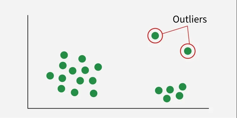 Outliers
- Impact on ML models: Can bias parameter estimation, increase variance and reduce model accuracy.
- Sources: Data entry errors, measurement noise, genuine rare events.
- Handling methods: Removal, transformation or robust algorithms less sensitive to outliers.
- Domain dependence: What is considered an outlier in one domain (e.g., finance) may be normal in another.
Types of Outliers
Outliers can be categorized as:
1. Global Outliers (Point Anomalies):
- Individual data points that lie far from the rest.
- Example: A wine record with alcohol level 20% when most are <15%.
2. Contextual Outliers:
- Outliers relative to a specific context or condition.
- Example: 30°C might be normal in summer but an outlier in winter.
3.Collective Outliers:
- A group of related data points behaving anomalously together.
- Example: A sudden spike in residual sugar and acidity in wine samples together.
Outliers Detection Methods
We will be using Wine Quality Dataset to illustrate different techniques.
The used dataset can be downloaded from here.
Step 1: Import Libraries and Load Dataset
Here we will import numpy, pandas, matplotlib, seaborn, scikit learn and scipy.
Python
import pandas as pd
import numpy as np
import matplotlib.pyplot as plt
import seaborn as sns
from sklearn.ensemble import IsolationForest
from sklearn.neighbors import LocalOutlierFactor
from scipy import stats

df = pd.read_csv("winequality-red.csv")
print(df.shape)
print(df.head())

data = df.drop("quality", axis=1)
Output:
 Dataset
Step 2: Visualize
Python
plt.figure(figsize=(12, 6))
sns.boxplot(data=data)
plt.xticks(rotation=45)
plt.title("Boxplots of Wine Features")
plt.show()
Output:
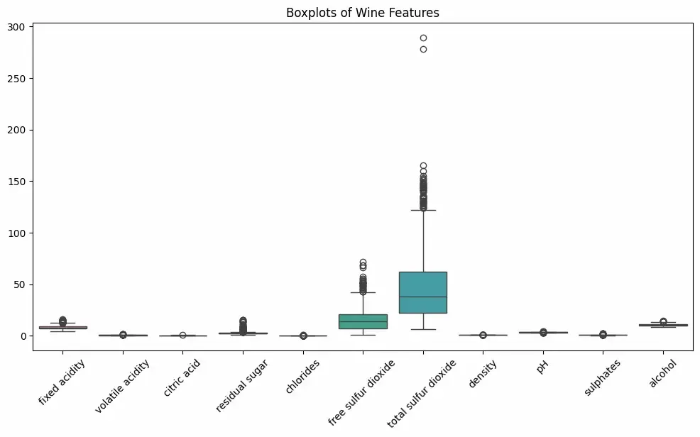 Boxplot
Here we can see black dots represents outliers in our dataset on which we will work now using different techniques like:
1. Z-Score Method
he Z-Score method is a statistical technique that detects outliers based on how far a data point is from the mean, measured in terms of standard deviations. It assumes the data follows a normal distribution. A point with a very high or low Z-score (typically |Z| > 3) is flagged as an outlier because it lies in the extreme tails of the distribution.
Formula:
Z = \frac{x - \mu}{\sigma}
Where,
- Z: The Z-score (standard score): It tells us how many standard deviations a data point is away from the mean.
- x: The actual data value (the observation we are testing).
- \mu : The mean of the dataset (average of all data points).
- \sigma: The standard deviation of the dataset (a measure of spread/variability).
How it works: Compares distance of a point from the mean in units of standard deviation.
- Intuition: Outliers are “too far” from the center of the bell curve.
- Pros: Simple, fast, works well with normally distributed data.
- Cons: Not reliable for skewed or non-normal distributions.
Python
z_scores = np.abs(stats.zscore(data))
outliers_z = np.where(z_scores > 3)

print("Outlier positions (row, col):")
print(list(zip(outliers_z[0][:10], outliers_z[1][:10])))
- stats.zscore(data) computes Z-scores for all columns.
- np.where(z_scores > 3) finds data points with |Z| > 3.
- We print the first few row-column indices where outliers occur.
Output:
Outlier positions (row, col):
[(np.int64(13), np.int64(9)), (np.int64(14), np.int64(5)), (np.int64(15), np.int64(5)), . . ., (np.int64(42), np.int64(4))]
2. IQR Method (Interquartile Range)
The IQR method is a robust statistical approach that identifies outliers by examining the spread of the middle 50% of the data. It calculates the Interquartile Range (IQR), which is the difference between the 75th percentile (Q3) and 25th percentile (Q1). Any value that falls below Q1 − 1.5 × IQR or above Q3 + 1.5 × IQR is considered an outlier.
Formula:
IQR = Q3 - Q1
Outliers Thresholds:
- \text{Lower bound} = Q1 - 1.5 \times IQR
- \text{Upper bound}= Q3 + 1.5 \times IQR
Intuition: Values too far below or above the “box” in a boxplot are flagged.
- Pros: Robust to non-normal data, less influenced by extreme values.
- Cons: Doesn’t adapt well to very skewed distributions.
Python
Q1 = data.quantile(0.25)
Q3 = data.quantile(0.75)
IQR = Q3 - Q1

outliers_iqr = ((data < (Q1 - 1.5 * IQR)) | (data > (Q3 + 1.5 * IQR)))
print("Number of outliers per column:")
print(outliers_iqr.sum())
- Compute Q1, Q3 and IQR for all columns.
- Create conditions to flag values below Q1 − 1.5 × IQR or above Q3 + 1.5 × IQR.
- Count flagged values per column.
Output:
 IQR Method
3. Isolation Forest
Isolation Forest is a model-based anomaly detection algorithm that isolates outliers instead of profiling normal data. It builds multiple random decision trees by repeatedly splitting the data. Since outliers are few and different, they are easier to isolate and require fewer splits.
How it works:
- Randomly select features and split values.
- Construct isolation trees.
- Compute average path length for each point.
- Shorter path = more likely outlier.
Pros: Works well in high dimensions, efficient.
Cons: Requires choosing contamination (expected outlier fraction).
Python
iso = IsolationForest(contamination=0.05, random_state=42)
y_pred_iso = iso.fit_predict(data)

df["IsoForest_Outlier"] = y_pred_iso
print(df["IsoForest_Outlier"].value_counts())

plt.figure(figsize=(7, 5))
sns.scatterplot(x="alcohol", y="residual sugar", data=df,
                hue="IsoForest_Outlier", palette="coolwarm")
plt.title("Isolation Forest Outlier Detection")
plt.show()
- contamination=0.05 assumes 5% of data are outliers.
- fit_predict() trains the forest and labels each point: -1 = outlier and 1 = normal
- Results are stored in a new column "IsoForest_Outlier".
Output:
IsoForest_Outlier
1 1519
-1 80
 Isolation Forest
 4. Local Outlier Factor (LOF)
The Local Outlier Factor (LOF) method is a density-based anomaly detection technique that compares the local density of a data point to that of its neighbors. If a point has significantly lower density than its neighbors, it is flagged as an outlier.
How it works:
- For each point, find k-nearest neighbors.
- Estimate local density based on neighbor distances.
- Compare the density of the point with its neighbors.
- If the point’s density ≪ neighbors → outlier.
Pros: Works well with clusters of varying density.
Cons: Sensitive to choice of k (neighbors).
Python
lof = LocalOutlierFactor(n_neighbors=20, contamination=0.05)
y_pred_lof = lof.fit_predict(data)

df["LOF_Outlier"] = y_pred_lof
print(df["LOF_Outlier"].value_counts())

plt.figure(figsize=(7, 5))
sns.scatterplot(x="alcohol", y="volatile acidity",
                data=df, hue="LOF_Outlier", palette="Set1")
plt.title("LOF Outlier Detection")
plt.show()
- n_neighbors=20 defines neighborhood size.
- fit_predict() assigns labels i.e -1 as outlier and 1 as normal
- Results are stored in "LOF_Outlier".
Output:
LOF_Outlier
1 1519
-1 80

Comparison of Outlier Detection Techniques
| Technique | Type | Key Idea | Works Well For | Pros | Cons |
|---|
| Z-Score | Statistical | Flags points far from mean (in SD units) | Normally distributed continuous data | Simple, fast and easy to implement | Not reliable for skewed or non-normal data |
|---|
| IQR | Statistical | Flags points outside 1.5×IQR from Q1/Q3 | Univariate data, boxplot-based analysis | Robust to extreme values and is non-parametric | Doesn’t adapt well to very skewed distributions |
|---|
| Isolation Forest | Model-based | Isolates outliers via random tree splits | High-dimensional datasets | Handles large datasets, efficient and works with many features | Requires setting contamination parameter with which results can vary |
|---|
| Local Outlier Factor (LOF) | Density-based | Compares local density to neighbors | Data with clusters or varying densities | Detects local outliers well | Sensitive to number of neighbors (k), computationally costlier |
|---|
Understanding Outliers -IQR and Z-Score
Explore
Machine Learning Basics
Python for Machine Learning
Feature Engineering
Supervised Learning
Unsupervised Learning
Model Evaluation and Tuning
Advanced Techniques
Machine Learning Practice