Linear regression is a type of supervised machine-learning algorithm that learns from the labelled datasets and maps the data points with most optimized linear functions which can be used for prediction on new datasets. It assumes that there is a linear relationship between the input and output, meaning the output changes at a constant rate as the input changes. This relationship is represented by a straight line.
For example we want to predict a student's exam score based on how many hours they studied. We observe that as students study more hours, their scores go up. In the example of predicting exam scores based on hours studied. Here
- Independent variable (input): Hours studied because it's the factor we control or observe.
- Dependent variable (output): Exam score because it depends on how many hours were studied.
We use the independent variable to predict the dependent variable.
Why Linear Regression is Important?
Here’s why linear regression is important:
- Simplicity and Interpretability: It’s easy to understand and interpret, making it a starting point for learning about machine learning.
- Predictive Ability: Helps predict future outcomes based on past data, making it useful in various fields like finance, healthcare and marketing.
- Basis for Other Models: Many advanced algorithms, like logistic regression or neural networks, build on the concepts of linear regression.
- Efficiency: It’s computationally efficient and works well for problems with a linear relationship.
- Widely Used: It’s one of the most widely used techniques in both statistics and machine learning for regression tasks.
- Analysis: It provides insights into relationships between variables (e.g., how much one variable influences another).
Best Fit Line in Linear Regression
In linear regression, the best-fit line is the straight line that most accurately represents the relationship between the independent variable (input) and the dependent variable (output). It is the line that minimizes the difference between the actual data points and the predicted values from the model.
1. Goal of the Best-Fit Line
The goal of linear regression is to find a straight line that minimizes the error (the difference) between the observed data points and the predicted values. This line helps us predict the dependent variable for new, unseen data.
 Linear Regression
Here Y is called a dependent or target variable and X is called an independent variable also known as the predictor of Y. There are many types of functions or modules that can be used for regression. A linear function is the simplest type of function. Here, X may be a single feature or multiple features representing the problem.
2. Equation of the Best-Fit Line
For simple linear regression (with one independent variable), the best-fit line is represented by the equation
y = mx + b
Where:
- y is the predicted value (dependent variable)
- x is the input (independent variable)
- m is the slope of the line (how much y changes when x changes)
- b is the intercept (the value of y when x = 0)
The best-fit line will be the one that optimizes the values of m (slope) and b (intercept) so that the predicted y values are as close as possible to the actual data points.
3. Minimizing the Error: The Least Squares Method
To find the best-fit line, we use a method called Least Squares. The idea behind this method is to minimize the sum of squared differences between the actual values (data points) and the predicted values from the line. These differences are called residuals.
The formula for residuals is:
Residual = yᵢ - ŷᵢ
Where:
- yᵢ is the actual observed value
- ŷᵢ is the predicted value from the line for that xᵢ
The least squares method minimizes the sum of the squared residuals:
Sum of squared errors (SSE) = Σ(yᵢ - ŷᵢ)²
This method ensures that the line best represents the data where the sum of the squared differences between the predicted values and actual values is as small as possible.
4. Interpretation of the Best-Fit Line
- Slope (m): The slope of the best-fit line indicates how much the dependent variable (y) changes with each unit change in the independent variable (x). For example if the slope is 5, it means that for every 1-unit increase in x, the value of y increases by 5 units.
- Intercept (b): The intercept represents the predicted value of y when x = 0. It’s the point where the line crosses the y-axis.
In linear regression some hypothesis are made to ensure reliability of the model's results.
Limitations
- Assumes Linearity: The method assumes the relationship between the variables is linear. If the relationship is non-linear, linear regression might not work well.
- Sensitivity to Outliers: Outliers can significantly affect the slope and intercept, skewing the best-fit line.
Hypothesis function in Linear Regression
In linear regression, the hypothesis function is the equation used to make predictions about the dependent variable based on the independent variables. It represents the relationship between the input features and the target output.
For a simple case with one independent variable, the hypothesis function is:
h(x) = β₀ + β₁x
Where:
- h(x) (or ŷ) is the predicted value of the dependent variable (y).
- x x is the independent variable.
- β₀ is the intercept, representing the value of y when x is 0.
- β₁ is the slope, indicating how much y changes for each unit change in x.
For multiple linear regression (with more than one independent variable), the hypothesis function expands to:
h(x₁, x₂, ..., xₖ) = β₀ + β₁x₁ + β₂x₂ + ... + βₖxₖ
Where:
- x₁, x₂, ..., xₖ are the independent variables.
- β₀ is the intercept.
- β₁, β₂, ..., βₖ are the coefficients, representing the influence of each respective independent variable on the predicted output.
Assumptions of the Linear Regression
1. Linearity: The relationship between inputs (X) and the output (Y) is a straight line.
 Linearity
2. Independence of Errors: The errors in predictions should not affect each other.
3. Constant Variance (Homoscedasticity): The errors should have equal spread across all values of the input. If the spread changes (like fans out or shrinks), it's called heteroscedasticity and it's a problem for the model.
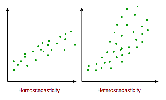 Homoscedasticity
4. Normality of Errors: The errors should follow a normal (bell-shaped) distribution.
5. No Multicollinearity(for multiple regression): Input variables shouldn’t be too closely related to each other.
6. No Autocorrelation: Errors shouldn't show repeating patterns, especially in time-based data.
7. Additivity: The total effect on Y is just the sum of effects from each X, no mixing or interaction between them.'
To understand Multicollinearityin detail refer to article: Multicollinearity.
Types of Linear Regression
When there is only one independent feature it is known as Simple Linear Regression or Univariate Linear Regression and when there are more than one feature it is known as Multiple Linear Regression or Multivariate Regression.
1. Simple Linear Regression
Simple linear regression is used when we want to predict a target value (dependent variable) using only one input feature (independent variable). It assumes a straight-line relationship between the two.
\hat{y} = \theta_0 + \theta_1 x
Where:
- \hat{y} is the predicted value
- x is the input (independent variable)
- \theta_0 is the intercept (value of \hat{y} when x=0)
- \theta_1 is the slope or coefficient (how much \hat{y} changes with one unit of x)
Example:
Predicting a person’s salary (y) based on their years of experience (x).
2. Multiple Linear Regression
Multiple linear regression involves more than one independent variable and one dependent variable. The equation for multiple linear regression is:
\hat{y} = \theta_0 + \theta_1 x_1 + \theta_2 x_2 + \cdots + \theta_n x_n
where:
- \hat{y} is the predicted value
- x_1, x_2, \dots, x_n \quad are the independent variables
- \theta_1, \theta_2, \dots, \theta_n \quad are the coefficients (weights) corresponding to each predictor.
- \theta_0 \quad is the intercept.
The goal of the algorithm is to find the best Fit Line equation that can predict the values based on the independent variables.
In regression set of records are present with X and Y values and these values are used to learn a function so if you want to predict Y from an unknown X this learned function can be used. In regression we have to find the value of Y, So, a function is required that predicts continuous Y in the case of regression given X as independent features.
Use Case of Multiple Linear Regression
Multiple linear regression allows us to analyze relationship between multiple independent variables and a single dependent variable. Here are some use cases:
- Real Estate Pricing: In real estate MLR is used to predict property prices based on multiple factors such as location, size, number of bedrooms, etc. This helps buyers and sellers understand market trends and set competitive prices.
- Financial Forecasting: Financial analysts use MLR to predict stock prices or economic indicators based on multiple influencing factors such as interest rates, inflation rates and market trends. This enables better investment strategies and risk management24.
- Agricultural Yield Prediction: Farmers can use MLR to estimate crop yields based on several variables like rainfall, temperature, soil quality and fertilizer usage. This information helps in planning agricultural practices for optimal productivity
- E-commerce Sales Analysis: An e-commerce company can utilize MLR to assess how various factors such as product price, marketing promotions and seasonal trends impact sales.
Now that we have understood about linear regression, its assumption and its type now we will learn how to make a linear regression model.
Cost function for Linear Regression
As we have discussed earlier about best fit line in linear regression, its not easy to get it easily in real life cases so we need to calculate errors that affects it. These errors need to be calculated to mitigate them. The difference between the predicted value \hat{Y} and the true value Y and it is called cost function or the loss function.
In Linear Regression, the Mean Squared Error (MSE) cost function is employed, which calculates the average of the squared errors between the predicted values \hat{y}_i and the actual values {y}_i. The purpose is to determine the optimal values for the intercept \theta_1 and the coefficient of the input feature \theta_2 providing the best-fit line for the given data points. The linear equation expressing this relationship is \hat{y}_i = \theta_1 + \theta_2x_i.
MSE function can be calculated as:
\text{Cost function}(J) = \frac{1}{n}\sum_{n}^{i}(\hat{y_i}-y_i)^2
Utilizing the MSE function, the iterative process of gradient descent is applied to update the values of \\theta_1 \& \theta_2 . This ensures that the MSE value converges to the global minima, signifying the most accurate fit of the linear regression line to the dataset.
This process involves continuously adjusting the parameters \(\theta_1\) and \(\theta_2\) based on the gradients calculated from the MSE. The final result is a linear regression line that minimizes the overall squared differences between the predicted and actual values, providing an optimal representation of the underlying relationship in the data.
Now we have calculated loss function we need to optimize model to mtigate this error and it is done through gradient descent.
Gradient Descent for Linear Regression
A linear regression model can be trained using the optimization algorithm gradient descent by iteratively modifying the model's parameters to reduce the mean squared error (MSE) of the model on a training dataset. To update θ1 and θ2 values in order to reduce the Cost function (minimizing RMSE value) and achieve the best-fit line the model uses Gradient Descent. The idea is to start with random θ1 and θ2 values and then iteratively update the values, reaching minimum cost.
A gradient is nothing but a derivative that defines the effects on outputs of the function with a little bit of variation in inputs.
Let's differentiate the cost function(J) with respect to \theta_1
\begin {aligned} {J}'_{\theta_1} &=\frac{\partial J(\theta_1,\theta_2)}{\partial \theta_1} \\ &= \frac{\partial}{\partial \theta_1} \left[\frac{1}{n} \left(\sum_{i=1}^{n}(\hat{y}_i-y_i)^2 \right )\right] \\ &= \frac{1}{n}\left[\sum_{i=1}^{n}2(\hat{y}_i-y_i) \left(\frac{\partial}{\partial \theta_1}(\hat{y}_i-y_i) \right ) \right] \\ &= \frac{1}{n}\left[\sum_{i=1}^{n}2(\hat{y}_i-y_i) \left(\frac{\partial}{\partial \theta_1}( \theta_1 + \theta_2x_i-y_i) \right ) \right] \\ &= \frac{1}{n}\left[\sum_{i=1}^{n}2(\hat{y}_i-y_i) \left(1+0-0 \right ) \right] \\ &= \frac{1}{n}\left[\sum_{i=1}^{n}(\hat{y}_i-y_i) \left(2 \right ) \right] \\ &= \frac{2}{n}\sum_{i=1}^{n}(\hat{y}_i-y_i) \end {aligned}
Let's differentiate the cost function(J) with respect to \theta_2
\begin {aligned} {J}'_{\theta_2} &=\frac{\partial J(\theta_1,\theta_2)}{\partial \theta_2} \\ &= \frac{\partial}{\partial \theta_2} \left[\frac{1}{n} \left(\sum_{i=1}^{n}(\hat{y}_i-y_i)^2 \right )\right] \\ &= \frac{1}{n}\left[\sum_{i=1}^{n}2(\hat{y}_i-y_i) \left(\frac{\partial}{\partial \theta_2}(\hat{y}_i-y_i) \right ) \right] \\ &= \frac{1}{n}\left[\sum_{i=1}^{n}2(\hat{y}_i-y_i) \left(\frac{\partial}{\partial \theta_2}( \theta_1 + \theta_2x_i-y_i) \right ) \right] \\ &= \frac{1}{n}\left[\sum_{i=1}^{n}2(\hat{y}_i-y_i) \left(0+x_i-0 \right ) \right] \\ &= \frac{1}{n}\left[\sum_{i=1}^{n}(\hat{y}_i-y_i) \left(2x_i \right ) \right] \\ &= \frac{2}{n}\sum_{i=1}^{n}(\hat{y}_i-y_i)\cdot x_i \end {aligned}
Finding the coefficients of a linear equation that best fits the training data is the objective of linear regression. By moving in the direction of the Mean Squared Error negative gradient with respect to the coefficients, the coefficients can be changed. And the respective intercept and coefficient of X will be if \alpha is the learning rate.
.webp) Gradient Descent
Gradient Descent\begin{aligned} \theta_1 &= \theta_1 - \alpha \left( {J}'_{\theta_1}\right) \\&=\theta_1 -\alpha \left( \frac{2}{n}\sum_{i=1}^{n}(\hat{y}_i-y_i)\right) \end{aligned} \\ \begin{aligned} \theta_2 &= \theta_2 - \alpha \left({J}'_{\theta_2}\right) \\&=\theta_2 - \alpha \left(\frac{2}{n}\sum_{i=1}^{n}(\hat{y}_i-y_i)\cdot x_i\right) \end{aligned}
After optimizing our model, we evaluate our models accuracy to see how well it will perform in real world scenario.
Evaluation Metrics for Linear Regression
A variety of evaluation measures can be used to determine the strength of any linear regression model. These assessment metrics often give an indication of how well the model is producing the observed outputs.
The most common measurements are:
1. Mean Square Error (MSE)
Mean Squared Error (MSE) is an evaluation metric that calculates the average of the squared differences between the actual and predicted values for all the data points. The difference is squared to ensure that negative and positive differences don't cancel each other out.
MSE = \frac{1}{n}\sum_{i=1}^{n}\left ( y_i - \widehat{y_{i}} \right )^2
Here,
- n is the number of data points.
- y_i is the actual or observed value for thei^{th} data point.
- \widehat{y_{i}}
is the predicted value for the i^{th} data point.
MSE is a way to quantify the accuracy of a model's predictions. MSE is sensitive to outliers as large errors contribute significantly to the overall score.
2. Mean Absolute Error (MAE)
Mean Absolute Error is an evaluation metric used to calculate the accuracy of a regression model. MAE measures the average absolute difference between the predicted values and actual values.
Mathematically MAE is expressed as:
MAE =\frac{1}{n} \sum_{i=1}^{n}|Y_i - \widehat{Y_i}|
Here,
- n is the number of observations
- Yi represents the actual values.
- \widehat{Y_i}
represents the predicted values
Lower MAE value indicates better model performance. It is not sensitive to the outliers as we consider absolute differences.
3. Root Mean Squared Error (RMSE)
The square root of the residuals' variance is the Root Mean Squared Error. It describes how well the observed data points match the expected values or the model's absolute fit to the data.
In mathematical notation, it can be expressed as:
RMSE=\sqrt{\frac{RSS}{n}}=\sqrt\frac{{{\sum_{i=2}^{n}(y^{actual}_{i}}- y_{i}^{predicted})^2}}{n}
Rather than dividing the entire number of data points in the model by the number of degrees of freedom, one must divide the sum of the squared residuals to obtain an unbiased estimate. Then, this figure is referred to as the Residual Standard Error (RSE).
In mathematical notation, it can be expressed as:
RMSE=\sqrt{\frac{RSS}{n}}=\sqrt\frac{{{\sum_{i=2}^{n}(y^{actual}_{i}}- y_{i}^{predicted})^2}}{(n-2)}
RSME is not as good of a metric as R-squared. Root Mean Squared Error can fluctuate when the units of the variables vary since its value is dependent on the variables' units (it is not a normalized measure).
4. Coefficient of Determination (R-squared)
R-Squared is a statistic that indicates how much variation the developed model can explain or capture. It is always in the range of 0 to 1. In general, the better the model matches the data, the greater the R-squared number.
In mathematical notation, it can be expressed as:
R^{2}=1-(^{\frac{RSS}{TSS}})
- Residual sum of Squares(RSS): The sum of squares of the residual for each data point in the plot or data is known as the residual sum of squares or RSS. It is a measurement of the difference between the output that was observed and what was anticipated.
RSS=\sum_{i=1}^{n}(y_{i}-b_{0}-b_{1}x_{i})^{2}
- Total Sum of Squares (TSS): The sum of the data points' errors from the answer variable's mean is known as the total sum of squares or TSS.
TSS=\sum_{i=1}^{n}(y-\overline{y_{i}})^2.
R squared metric is a measure of the proportion of variance in the dependent variable that is explained the independent variables in the model.
5. Adjusted R-Squared Error
Adjusted R^2 measures the proportion of variance in the dependent variable that is explained by independent variables in a regression model. Adjusted R-square accounts the number of predictors in the model and penalizes the model for including irrelevant predictors that don't contribute significantly to explain the variance in the dependent variables.
Mathematically, adjusted R^2 is expressed as:
Adjusted \, R^2 = 1 - (\frac{(1-R^2).(n-1)}{n-k-1})
Here,
- n is the number of observations
- k is the number of predictors in the model
- R2 is coeeficient of determination
Adjusted R-square helps to prevent overfitting. It penalizes the model with additional predictors that do not contribute significantly to explain the variance in the dependent variable.
While evaluation metrics help us measure the performance of a model, regularization helps in improving that performance by addressing overfitting and enhancing generalization.
Regularization Techniques for Linear Models
1. Lasso Regression (L1 Regularization)
Lasso Regression is a technique used for regularizing a linear regression model, it adds a penalty term to the linear regression objective function to prevent overfitting.
The objective function after applying lasso regression is:
J(\theta) = \frac{1}{2m} \sum_{i=1}^{m}(\widehat{y_i} - y_i) ^2+ \lambda \sum_{j=1}^{n}|\theta_j|
- the first term is the least squares loss, representing the squared difference between predicted and actual values.
- the second term is the L1 regularization term, it penalizes the sum of absolute values of the regression coefficient θj.
2. Ridge Regression (L2 Regularization)
Ridge regression is a linear regression technique that adds a regularization term to the standard linear objective. Again, the goal is to prevent overfitting by penalizing large coefficient in linear regression equation. It useful when the dataset has multicollinearity where predictor variables are highly correlated.
The objective function after applying ridge regression is:
J(\theta) = \frac{1}{2m} \sum_{i=1}^{m}(\widehat{y_i} - y_i)^2 + \lambda \sum_{j=1}^{n}\theta_{j}^{2}
- the first term is the least squares loss, representing the squared difference between predicted and actual values.
- the second term is the L1 regularization term, it penalizes the sum of square of values of the regression coefficient θj.
3. Elastic Net Regression
Elastic Net Regression is a hybrid regularization technique that combines the power of both L1 and L2 regularization in linear regression objective.
J(\theta) = \frac{1}{2m} \sum_{i=1}^{m}(\widehat{y_i} - y_i)^2 + \alpha \lambda \sum_{j=1}^{n}{|\theta_j|} + \frac{1}{2}(1- \alpha) \lambda \sum_{j=1}{n} \theta_{j}^{2}
- the first term is least square loss.
- the second term is L1 regularization and third is ridge regression.
- \lambda is the overall regularization strength.
- \alpha controls the mix between L1 and L2 regularization.
Now that we have learned how to make a linear regression model, now we will implement it.
Python Implementation of Linear Regression
1. Import the necessary libraries:
Python
import pandas as pd
import numpy as np
import matplotlib.pyplot as plt
import matplotlib.axes as ax
from matplotlib.animation import FuncAnimation
Here is the link for dataset: Dataset Link
Python
url = 'https://media.geeksforgeeks.org/wp-content/uploads/20240320114716/data_for_lr.csv'
data = pd.read_csv(url)

data = data.dropna()

train_input = np.array(data.x[0:500]).reshape(500, 1)
train_output = np.array(data.y[0:500]).reshape(500, 1)

test_input = np.array(data.x[500:700]).reshape(199, 1)
test_output = np.array(data.y[500:700]).reshape(199, 1)
3. Build the Linear Regression Model and Plot the regression line
In forward propagation Linear regression function Y=mx+c is applied by initially assigning random value of parameter (m and c). The we have written the function to finding the cost function i.e the mean
Python
class LinearRegression:
    def __init__(self):
        self.parameters = {}

    def forward_propagation(self, train_input):
        m = self.parameters['m']
        c = self.parameters['c']
        predictions = np.multiply(m, train_input) + c
        return predictions

    def cost_function(self, predictions, train_output):
        cost = np.mean((train_output - predictions) ** 2)
        return cost

    def backward_propagation(self, train_input, train_output, predictions):
        derivatives = {}
        df = (predictions-train_output)
        dm = 2 * np.mean(np.multiply(train_input, df))
        dc = 2 * np.mean(df)
        derivatives['dm'] = dm
        derivatives['dc'] = dc
        return derivatives

    def update_parameters(self, derivatives, learning_rate):
        self.parameters['m'] = self.parameters['m'] - learning_rate * derivatives['dm']
        self.parameters['c'] = self.parameters['c'] - learning_rate * derivatives['dc']

    def train(self, train_input, train_output, learning_rate, iters):
        self.parameters['m'] = np.random.uniform(0, 1) * -1
        self.parameters['c'] = np.random.uniform(0, 1) * -1

        self.loss = []

        fig, ax = plt.subplots()
        x_vals = np.linspace(min(train_input), max(train_input), 100)
        line, = ax.plot(x_vals, self.parameters['m'] * x_vals + self.parameters['c'], color='red', label='Regression Line')
        ax.scatter(train_input, train_output, marker='o', color='green', label='Training Data')

        ax.set_ylim(0, max(train_output) + 1)

        def update(frame):
            predictions = self.forward_propagation(train_input)
            cost = self.cost_function(predictions, train_output)
            derivatives = self.backward_propagation(train_input, train_output, predictions)
            self.update_parameters(derivatives, learning_rate)
            line.set_ydata(self.parameters['m'] * x_vals + self.parameters['c'])
            self.loss.append(cost)
            print("Iteration = {}, Loss = {}".format(frame + 1, cost))
            return line,

        ani = FuncAnimation(fig, update, frames=iters, interval=200, blit=True)
        ani.save('linear_regression_A.gif', writer='ffmpeg')

        plt.xlabel('Input')
        plt.ylabel('Output')
        plt.title('Linear Regression')
        plt.legend()
        plt.show()

        return self.parameters, self.loss

The linear regression line provides valuable insights into the relationship between the two variables. It represents the best-fitting line that captures the overall trend of how a dependent variable (Y) changes in response to variations in an independent variable (X).
- Positive Linear Regression Line: A positive linear regression line indicates a direct relationship between the independent variable (X) and the dependent variable (Y). This means that as the value of X increases, the value of Y also increases. The slope of a positive linear regression line is positive, meaning that the line slants upward from left to right.
- Negative Linear Regression Line: A negative linear regression line indicates an inverse relationship between the independent variable (X) and the dependent variable (Y ). This means that as the value of X increases, the value of Y decreases. The slope of a negative linear regression line is negative, meaning that the line slants downward from left to right.
4. Trained the model and Final Prediction
Python
linear_reg = LinearRegression()
parameters, loss = linear_reg.train(train_input, train_output, 0.0001, 20)
Output:
 Model Training
Applications of Linear Regression
Linear regression is used in many different fields including finance, economics and psychology to understand and predict the behavior of a particular variable.
For example linear regression is widely used in finance to analyze relationships and make predictions. It can model how a company's earnings per share (EPS) influence its stock price. If the model shows that a $1 increase in EPS results in a $15 rise in stock price, investors gain insights into the company's valuation. Similarly, linear regression can forecast currency values by analyzing historical exchange rates and economic indicators, helping financial professionals make informed decisions and manage risks effectively.
Also read - Linear Regression - In Simple Words, with real-life Examples
Advantages and Disadvantages of Linear Regression
Advantages of Linear Regression
- Linear regression is a relatively simple algorithm, making it easy to understand and implement. The coefficients of the linear regression model can be interpreted as the change in the dependent variable for a one-unit change in the independent variable, providing insights into the relationships between variables.
- Linear regression is computationally efficient and can handle large datasets effectively. It can be trained quickly on large datasets, making it suitable for real-time applications.
- Linear regression is relatively robust to outliers compared to other machine learning algorithms. Outliers may have a smaller impact on the overall model performance.
- Linear regression often serves as a good baseline model for comparison with more complex machine learning algorithms.
- Linear regression is a well-established algorithm with a rich history and is widely available in various machine learning libraries and software packages.
Disadvantages of Linear Regression
- Linear regression assumes a linear relationship between the dependent and independent variables. If the relationship is not linear, the model may not perform well.
- Linear regression is sensitive to multicollinearity, which occurs when there is a high correlation between independent variables. Multicollinearity can inflate the variance of the coefficients and lead to unstable model predictions.
- Linear regression assumes that the features are already in a suitable form for the model. Feature engineering may be required to transform features into a format that can be effectively used by the model.
- Linear regression is susceptible to both overfitting and underfitting. Overfitting occurs when the model learns the training data too well and fails to generalize to unseen data. Underfitting occurs when the model is too simple to capture the underlying relationships in the data.
- Linear regression provides limited explanatory power for complex relationships between variables. More advanced machine learning techniques may be necessary for deeper insights.
Similar Reads
Maths for Machine Learning Mathematics is the foundation of machine learning. Math concepts plays a crucial role in understanding how models learn from data and optimizing their performance. Before diving into machine learning algorithms, it's important to familiarize yourself with foundational topics, like Statistics, Probab
5 min read
Linear Algebra and Matrix
MatricesMatrices are key concepts in mathematics, widely used in solving equations and problems in fields like physics and computer science. A matrix is simply a grid of numbers, and a determinant is a value calculated from a square matrix.Example: \begin{bmatrix} 6 & 9 \\ 5 & -4 \\ \end{bmatrix}_{2
3 min read
Scalar and VectorScalar and Vector Quantities are used to describe the motion of an object. Scalar Quantities are defined as physical quantities that have magnitude or size only. For example, distance, speed, mass, density, etc.However, vector quantities are those physical quantities that have both magnitude and dir
8 min read
Add Two Matrices - PythonThe task of adding two matrices in Python involves combining corresponding elements from two given matrices to produce a new matrix. Each element in the resulting matrix is obtained by adding the values at the same position in the input matrices. For example, if two 2x2 matrices are given as:Two 2x2
3 min read
Python Program to Multiply Two MatricesGiven two matrices, we will have to create a program to multiply two matrices in Python. Example: Python Matrix Multiplication of Two-DimensionPythonmatrix_a = [[1, 2], [3, 4]] matrix_b = [[5, 6], [7, 8]] result = [[0, 0], [0, 0]] for i in range(2): for j in range(2): result[i][j] = (matrix_a[i][0]
5 min read
Vector OperationsVectors are fundamental quantities in physics and mathematics, that have both magnitude and direction. So performing mathematical operations on them directly is not possible. So we have special operations that work only with vector quantities and hence the name, vector operations. Thus, It is essent
8 min read
Product of VectorsVector operations are used almost everywhere in the field of physics. Many times these operations include addition, subtraction, and multiplication. Addition and subtraction can be performed using the triangle law of vector addition. In the case of products, vector multiplication can be done in two
5 min read
Scalar Product of VectorsTwo vectors or a vector and a scalar can be multiplied. There are mainly two kinds of products of vectors in physics, scalar multiplication of vectors and Vector Product (Cross Product) of two vectors. The result of the scalar product of two vectors is a number (a scalar). The common use of the scal
9 min read
Dot and Cross Products on VectorsA quantity that has both magnitude and direction is known as a vector. Various operations can be performed on such quantities, such as addition, subtraction, and multiplication (products), etc. Some examples of vector quantities are: velocity, force, acceleration, and momentum, etc.Vectors can be mu
8 min read
Transpose a matrix in Single line in PythonTranspose of a matrix is a task we all can perform very easily in Python (Using a nested loop). But there are some interesting ways to do the same in a single line. In Python, we can implement a matrix as a nested list (a list inside a list). Each element is treated as a row of the matrix. For examp
4 min read
Transpose of a MatrixA Matrix is a rectangular arrangement of numbers (or elements) in rows and columns. It is often used in mathematics to represent data, solve systems of equations, or perform transformations. A matrix is written as:A = \begin{bmatrix} 1 & 2 & 3\\ 4 & 5 & 6 \\ 7 & 8 & 9\end{bma
11 min read
Adjoint and Inverse of a MatrixGiven a square matrix, find the adjoint and inverse of the matrix. We strongly recommend you to refer determinant of matrix as a prerequisite for this. Adjoint (or Adjugate) of a matrix is the matrix obtained by taking the transpose of the cofactor matrix of a given square matrix is called its Adjoi
15+ min read
How to inverse a matrix using NumPyIn this article, we will see NumPy Inverse Matrix in Python before that we will try to understand the concept of it. The inverse of a matrix is just a reciprocal of the matrix as we do in normal arithmetic for a single number which is used to solve the equations to find the value of unknown variable
3 min read
Program to find Determinant of a MatrixThe determinant of a Matrix is defined as a special number that is defined only for square matrices (matrices that have the same number of rows and columns). A determinant is used in many places in calculus and other matrices related to algebra, it actually represents the matrix in terms of a real n
15+ min read
Program to find Normal and Trace of a matrixGiven a 2D matrix, the task is to find Trace and Normal of matrix.Normal of a matrix is defined as square root of sum of squares of matrix elements.Trace of a n x n square matrix is sum of diagonal elements. Examples : Input : mat[][] = {{7, 8, 9}, {6, 1, 2}, {5, 4, 3}}; Output : Normal = 16 Trace =
6 min read
Data Science | Solving Linear EquationsLinear Algebra is a very fundamental part of Data Science. When one talks about Data Science, data representation becomes an important aspect of Data Science. Data is represented usually in a matrix form. The second important thing in the perspective of Data Science is if this data contains several
8 min read
Data Science - Solving Linear Equations with PythonA collection of equations with linear relationships between the variables is known as a system of linear equations. The objective is to identify the values of the variables that concurrently satisfy each equation, each of which is a linear constraint. By figuring out the system, we can learn how the
4 min read
System of Linear EquationsIn mathematics, a system of linear equations consists of two or more linear equations that share the same variables. These systems often arise in real-world applications, such as engineering, physics, economics, and more, where relationships between variables need to be analyzed. Understanding how t
8 min read
System of Linear Equations in three variables using Cramer's RuleCramer's rule: In linear algebra, Cramer's rule is an explicit formula for the solution of a system of linear equations with as many equations as unknown variables. It expresses the solution in terms of the determinants of the coefficient matrix and of matrices obtained from it by replacing one colu
12 min read
Eigenvalues and EigenvectorsEigenvectors are the directions that remain unchanged during a transformation, even if they get longer or shorter. Eigenvalues are the numbers that indicate how much something stretches or shrinks during that transformation. These ideas are important in many areas of math and engineering, including
15+ min read
Applications of Eigenvalues and EigenvectorsEigenvalues and eigenvectors play a crucial role in a wide range of applications across engineering and science. Fields like control theory, vibration analysis, electric circuits, advanced dynamics, and quantum mechanics frequently rely on these concepts. One key application involves transforming ma
7 min read
How to compute the eigenvalues and right eigenvectors of a given square array using NumPY?In this article, we will discuss how to compute the eigenvalues and right eigenvectors of a given square array using NumPy library. Example: Suppose we have a matrix as: [[1,2], [2,3]] Eigenvalue we get from this matrix or square array is: [-0.23606798 4.23606798] Eigenvectors of this matrix are
2 min read
Statistics for Machine Learning
Descriptive StatisticStatistics is the foundation of data science. Descriptive statistics are simple tools that help us understand and summarize data. They show the basic features of a dataset, like the average, highest and lowest values and how spread out the numbers are. It's the first step in making sense of informat
5 min read
Measures of Central TendencyUsually, frequency distribution and graphical representation are used to depict a set of raw data to attain meaningful conclusions from them. However, sometimes, these methods fail to convey a proper and clear picture of the data as expected. Therefore, some measures, also known as Measures of Centr
5 min read
Measures of Dispersion | Types, Formula and ExamplesMeasures of Dispersion are used to represent the scattering of data. These are the numbers that show the various aspects of the data spread across multiple parameters.Let's learn about the measure of dispersion in statistics, its types, formulas, and examples in detail.Dispersion in StatisticsDisper
9 min read
Mean, Variance and Standard DeviationMean, Variance and Standard Deviation are fundamental concepts in statistics and engineering mathematics, essential for analyzing and interpreting data. These measures provide insights into data's central tendency, dispersion, and spread, which are crucial for making informed decisions in various en
10 min read
Calculate the average, variance and standard deviation in Python using NumPyNumpy in Python is a general-purpose array-processing package. It provides a high-performance multidimensional array object and tools for working with these arrays. It is the fundamental package for scientific computing with Python. Numpy provides very easy methods to calculate the average, variance
5 min read
Random VariableRandom variable is a fundamental concept in statistics that bridges the gap between theoretical probability and real-world data. A Random variable in statistics is a function that assigns a real value to an outcome in the sample space of a random experiment. For example: if you roll a die, you can a
10 min read
Difference between Parametric and Non-Parametric MethodsStatistical analysis plays a crucial role in understanding and interpreting data across various disciplines. Two prominent approaches in statistical analysis are Parametric and Non-Parametric Methods. While both aim to draw inferences from data, they differ in their assumptions and underlying princi
8 min read
Probability Distribution - Function, Formula, TableA probability distribution is a mathematical function or rule that describes how the probabilities of different outcomes are assigned to the possible values of a random variable. It provides a way of modeling the likelihood of each outcome in a random experiment.While a frequency distribution shows
15+ min read
Confidence IntervalA Confidence Interval (CI) is a range of values that contains the true value of something we are trying to measure like the average height of students or average income of a population.Instead of saying: “The average height is 165 cm.â€We can say: “We are 95% confident the average height is between 1
7 min read
Covariance and CorrelationCovariance and correlation are the two key concepts in Statistics that help us analyze the relationship between two variables. Covariance measures how two variables change together, indicating whether they move in the same or opposite directions. Relationship between Independent and dependent variab
5 min read
Program to Find Correlation CoefficientThe correlation coefficient is a statistical measure that helps determine the strength and direction of the relationship between two variables. It quantifies how changes in one variable correspond to changes in another. This coefficient, sometimes referred to as the cross-correlation coefficient, al
8 min read
Robust CorrelationCorrelation is a statistical tool that is used to analyze and measure the degree of relationship or degree of association between two or more variables. There are generally three types of correlation: Positive correlation: When we increase the value of one variable, the value of another variable inc
8 min read
Normal Probability PlotThe probability plot is a way of visually comparing the data coming from different distributions. These data can be of empirical dataset or theoretical dataset. The probability plot can be of two types:P-P plot: The (Probability-to-Probability) p-p plot is the way to visualize the comparing of cumul
3 min read
Quantile Quantile plotsThe quantile-quantile( q-q plot) plot is a graphical method for determining if a dataset follows a certain probability distribution or whether two samples of data came from the same population or not. Q-Q plots are particularly useful for assessing whether a dataset is normally distributed or if it
8 min read
True Error vs Sample ErrorTrue Error The true error can be said as the probability that the hypothesis will misclassify a single randomly drawn sample from the population. Here the population represents all the data in the world. Let's consider a hypothesis h(x) and the true/target function is f(x) of population P. The proba
3 min read
Bias-Variance Trade Off - Machine LearningIt is important to understand prediction errors (bias and variance) when it comes to accuracy in any machine-learning algorithm. There is a tradeoff between a model’s ability to minimize bias and variance which is referred to as the best solution for selecting a value of Regularization constant. A p
3 min read
Hypothesis TestingHypothesis testing compares two opposite ideas about a group of people or things and uses data from a small part of that group (a sample) to decide which idea is more likely true. We collect and study the sample data to check if the claim is correct.Hypothesis TestingFor example, if a company says i
9 min read
T-testAfter learning about the Z-test we now move on to another important statistical test called the t-test. While the Z-test is useful when we know the population variance. The t-test is used to compare the averages of two groups to see if they are significantly different from each other. Suppose you wa
6 min read
Paired T-Test - A Detailed OverviewStudent’s t-test or t-test is the statistical method used to determine if there is a difference between the means of two samples. The test is often performed to find out if there is any sampling error or unlikeliness in the experiment. This t-test is further divided into 3 types based on your data a
5 min read
P-value in Machine LearningP-value helps us determine how likely it is to get a particular result when the null hypothesis is assumed to be true. It is the probability of getting a sample like ours or more extreme than ours if the null hypothesis is correct. Therefore, if the null hypothesis is assumed to be true, the p-value
6 min read
F-Test in StatisticsF test is a statistical test that is used in hypothesis testing that determines whether the variances of two samples are equal or not. The article will provide detailed information on f test, f statistic, its calculation, critical value and how to use it to test hypotheses. To understand F test firs
6 min read
Z-test : Formula, Types, ExamplesA Z-test is a type of hypothesis test that compares the sample’s average to the population’s average and calculates the Z-score and tells us how much the sample average is different from the population average by looking at how much the data normally varies. It is particularly useful when the sample
8 min read
Residual Leverage Plot (Regression Diagnostic)In linear or multiple regression, it is not enough to just fit the model into the dataset. But, it may not give the desired result. To apply the linear or multiple regression efficiently to the dataset. There are some assumptions that we need to check on the dataset that made linear/multiple regress
5 min read
Difference between Null and Alternate HypothesisHypothesis is a statement or an assumption that may be true or false. There are six types of hypotheses mainly the Simple hypothesis, Complex hypothesis, Directional hypothesis, Associative hypothesis, and Null hypothesis. Usually, the hypothesis is the start point of any scientific investigation, I
3 min read
Mann and Whitney U testMann and Whitney's U-test or Wilcoxon rank-sum testis the non-parametric statistic hypothesis test that is used to analyze the difference between two independent samples of ordinal data. In this test, we have provided two randomly drawn samples and we have to verify whether these two samples is from
5 min read
Wilcoxon Signed Rank TestThe Wilcoxon Signed Rank Test is a non-parametric statistical test used to compare two related groups. It is often applied when the assumptions for the paired t-test (such as normality) are not met. This test evaluates whether there is a significant difference between two paired observations, making
5 min read
Kruskal Wallis TestThe Kruskal-Wallis test (H test) is a nonparametric statistical test used to compare three or more independent groups to determine if there are statistically significant differences between them. It is an extension of the Mann-Whitney U test, which is used for comparing two groups.Unlike the one-way
4 min read
Friedman TestThe Friedman Test is a non-parametric statistical test used to detect differences in treatments across multiple test attempts. It is often used when the data is in the form of rankings or ordinal data, and when you have more than two related groups or repeated measures. The Friedman test is the non-
6 min read
Probability Class 10 Important QuestionsProbability is a fundamental concept in mathematics for measuring of chances of an event happening By assigning numerical values to the chances of different outcomes, probability allows us to model, analyze, and predict complex systems and processes.Probability Formulas for Class 10 It says the poss
4 min read
Probability and Probability Distributions
Mathematics - Law of Total ProbabilityProbability theory is the branch of mathematics concerned with the analysis of random events. It provides a framework for quantifying uncertainty, predicting outcomes, and understanding random phenomena. In probability theory, an event is any outcome or set of outcomes from a random experiment, and
12 min read
Bayes's Theorem for Conditional ProbabilityBayes's Theorem for Conditional Probability: Bayes's Theorem is a fundamental result in probability theory that describes how to update the probabilities of hypotheses when given evidence. Named after the Reverend Thomas Bayes, this theorem is crucial in various fields, including engineering, statis
9 min read
Uniform Distribution in Data ScienceUniform Distribution also known as the Rectangular Distribution is a type of Continuous Probability Distribution where all outcomes in a given interval are equally likely. Unlike Normal Distribution which have varying probabilities across their range, Uniform Distribution has a constant probability
5 min read
Binomial Distribution in Data ScienceBinomial Distribution is used to calculate the probability of a specific number of successes in a fixed number of independent trials where each trial results in one of two outcomes: success or failure. It is used in various fields such as quality control, election predictions and medical tests to ma
7 min read
Poisson Distribution in Data SciencePoisson Distribution is a discrete probability distribution that models the number of events occurring in a fixed interval of time or space given a constant average rate of occurrence. Unlike the Binomial Distribution which is used when the number of trials is fixed, the Poisson Distribution is used
7 min read
Uniform Distribution | Formula, Definition and ExamplesA Uniform Distribution is a type of probability distribution in which every outcome in a given range is equally likely to occur. That means there is no bias—no outcome is more likely than another within the specified set.It is also known as rectangular distribution (continuous uniform distribution).
11 min read
Exponential DistributionThe Exponential Distribution is one of the most commonly used probability distributions in statistics and data science. It is widely used to model the time or space between events in a Poisson process. In simple terms, it describes how long you have to wait before something happens, like a bus arriv
3 min read
Normal Distribution in Data ScienceNormal Distribution also known as the Gaussian Distribution or Bell-shaped Distribution is one of the widely used probability distributions in statistics. It plays an important role in probability theory and statistics basically in the Central Limit Theorem (CLT). It is characterized by its bell-sha
6 min read
Mathematics | Beta Distribution ModelThe Beta Distribution is a continuous probability distribution defined on the interval [0, 1], widely used in statistics and various fields for modeling random variables that represent proportions or probabilities. It is particularly useful when dealing with scenarios where the outcomes are bounded
11 min read
Gamma Distribution Model in MathematicsIntroduction : Suppose an event can occur several times within a given unit of time. When the total number of occurrences of the event is unknown, we can think of it as a random variable. Now, if this random variable X has gamma distribution, then its probability density function is given as follows
2 min read
Chi-Square Test for Feature Selection - Mathematical ExplanationOne of the primary tasks involved in any supervised Machine Learning venture is to select the best features from the given dataset to obtain the best results. One way to select these features is the Chi-Square Test. Mathematically, a Chi-Square test is done on two distributions two determine the lev
4 min read
Student's t-distribution in StatisticsAs we know normal distribution assumes two important characteristics about the dataset: a large sample size and knowledge of the population standard deviation. However, if we do not meet these two criteria, and we have a small sample size or an unknown population standard deviation, then we use the
10 min read
Python - Central Limit TheoremCentral Limit Theorem (CLT) is a foundational principle in statistics, and implementing it using Python can significantly enhance data analysis capabilities. Statistics is an important part of data science projects. We use statistical tools whenever we want to make any inference about the population
7 min read
Limits, Continuity and DifferentiabilityLimits, Continuity, and Differentiation are fundamental concepts in calculus. They are essential for analyzing and understanding function behavior and are crucial for solving real-world problems in physics, engineering, and economics.Table of ContentLimitsKey Characteristics of LimitsExample of Limi
10 min read
Implicit DifferentiationImplicit Differentiation is the process of differentiation in which we differentiate the implicit function without converting it into an explicit function. For example, we need to find the slope of a circle with an origin at 0 and a radius r. Its equation is given as x2 + y2 = r2. Now, to find the s
5 min read
Calculus for Machine Learning
Partial Derivatives in Engineering MathematicsPartial derivatives are a basic concept in multivariable calculus. They convey how a function would change when one of its input variables changes, while keeping all the others constant. This turns out to be particularly useful in fields such as physics, engineering, economics, and computer science,
10 min read
Advanced DifferentiationDerivatives are used to measure the rate of change of any quantity. This process is called differentiation. It can be considered as a building block of the theory of calculus. Geometrically speaking, the derivative of any function at a particular point gives the slope of the tangent at that point of
8 min read
How to find Gradient of a Function using Python?The gradient of a function simply means the rate of change of a function. We will use numdifftools to find Gradient of a function. Examples: Input : x^4+x+1 Output :Gradient of x^4+x+1 at x=1 is 4.99 Input :(1-x)^2+(y-x^2)^2 Output :Gradient of (1-x^2)+(y-x^2)^2 at (1, 2) is [-4. 2.] Approach: For S
2 min read
Optimization techniques for Gradient DescentGradient Descent is a widely used optimization algorithm for machine learning models. However, there are several optimization techniques that can be used to improve the performance of Gradient Descent. Here are some of the most popular optimization techniques for Gradient Descent: Learning Rate Sche
4 min read
Higher Order DerivativesHigher order derivatives refer to the derivatives of a function that are obtained by repeatedly differentiating the original function.The first derivative of a function, f′(x), represents the rate of change or slope of the function at a point.The second derivative, f′′(x), is the derivative of the f
6 min read
Taylor SeriesA Taylor series represents a function as an infinite sum of terms, calculated from the values of its derivatives at a single point.Taylor series is a powerful mathematical tool used to approximate complex functions with an infinite sum of terms derived from the function's derivatives at a single poi
8 min read
Application of Derivative - Maxima and MinimaDerivatives have many applications, like finding rate of change, approximation, maxima/minima and tangent. In this section, we focus on their use in finding maxima and minima.Note: If f(x) is a continuous function, then for every continuous function on a closed interval has a maximum and a minimum v
6 min read
Absolute Minima and MaximaAbsolute Maxima and Minima are the maximum and minimum values of the function defined on a fixed interval. A function in general can have high values or low values as we move along the function. The maximum value of the function in any interval is called the maxima and the minimum value of the funct
11 min read
Optimization for Data ScienceFrom a mathematical foundation viewpoint, it can be said that the three pillars for data science that we need to understand quite well are Linear Algebra, Statistics and the third pillar is Optimization which is used pretty much in all data science algorithms. And to understand the optimization conc
5 min read
Unconstrained Multivariate OptimizationWikipedia defines optimization as a problem where you maximize or minimize a real function by systematically choosing input values from an allowed set and computing the value of the function. That means when we talk about optimization we are always interested in finding the best solution. So, let sa
4 min read
Lagrange Multipliers | Definition and ExamplesIn mathematics, a Lagrange multiplier is a potent tool for optimization problems and is applied especially in the cases of constraints. Named after the Italian-French mathematician Joseph-Louis Lagrange, the method provides a strategy to find maximum or minimum values of a function along one or more
8 min read
Lagrange's InterpolationWhat is Interpolation? Interpolation is a method of finding new data points within the range of a discrete set of known data points (Source Wiki). In other words interpolation is the technique to estimate the value of a mathematical function, for any intermediate value of the independent variable. F
7 min read
Linear Regression in Machine learningLinear regression is a type of supervised machine-learning algorithm that learns from the labelled datasets and maps the data points with most optimized linear functions which can be used for prediction on new datasets. It assumes that there is a linear relationship between the input and output, mea
15+ min read
Ordinary Least Squares (OLS) using statsmodelsOrdinary Least Squares (OLS) is a widely used statistical method for estimating the parameters of a linear regression model. It minimizes the sum of squared residuals between observed and predicted values. In this article we will learn how to implement Ordinary Least Squares (OLS) regression using P
3 min read
Regression in Machine Learning