What is BM25 (Best Matching 25) Algorithm
Last Updated :
04 Nov, 2025
BM25 (Best Matching 25) is a ranking algorithm used in information retrieval systems to determine how relevant a document is to a given search query. It’s an improved version of the traditional TF-IDF (Term Frequency–Inverse Document Frequency) approach and is widely used in modern search engines and databases.
- It measures term frequency and document relevance more accurately.
- It accounts for document length normalization, giving fair weight to all documents.
- It is widely used in tools like Elasticsearch, Whoosh and Lucene.
- It helps to deliver more relevant search results based on keyword matching and context.
In simple terms, BM25 helps rank documents or web pages based on how well they match a user’s search terms making it a cornerstone of effective search and retrieval systems.
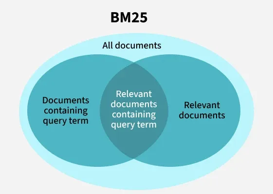 Overview of BM25
Working of BM25
BM25 computes a relevance score between a query q and a document d using three main components: Term Frequency (TF), Inverse Document Frequency (IDF) and Document Length Normalization.
1. Term Frequency (TF)
Term frequency measures how often a query term appears in a document. Intuitively, a document containing a query term multiple times is more likely to be relevant. However, BM25 introduces a saturation effect i.e beyond a certain point, additional occurrences of a term contribute less to the score. This prevents overly long documents from being unfairly favored.
Mathematically, the term frequency component is normalized using the formula:
TF(t,d)=\frac{freq(t,d)}{freq(t,d) + k_1 . (1-b+b.\frac{|d|}{\text{avgdl}})}
where:
- t: Query term
- d: Document
- freq(t,d): Number of times term t appears in document d
- ∣d∣: Length of document d
- \text{avgdl}: average document length in corpus
- k_1: controls term frequency scaling
- b: controls document length normalization
2. Inverse Document Frequency (IDF)
Inverse document frequency measures the importance of a term across the entire corpus. Rare terms are considered more informative than common ones. For example, the word "the" appears in almost every document and thus carries little value, whereas a rare term like "quantum" is more indicative of relevance.
The IDF component is calculated as:
IDF(t)=log(\frac{N-n_t+0.5}{n_t+0.5})
where:
- N: Total number of documents in the corpus
- n_t: Number of documents containing term t
3. Document Length Normalization
BM25 accounts for document length by normalizing scores to prevent longer documents from dominating the rankings. This is controlled by the parameter b which adjusts the influence of document length relative to the average document length (\text{avgdl}).
4. Final Score Calculation
The final BM25 score for a document d with respect to a query q is computed as:
Score(q,d) = \sum_{t\epsilon q}IDF(t).TF(t,d)
This sums up the contributions of all query terms t in the document d.
BM25 vs. Modern Dense Retrieval
Let's see the comparison between BM25 and Modern Dense Retrieval.
| Aspect | BM25 (Sparse/Term-based) | Dense/Embedding-based Retrieval |
|---|
| Representation | Term / lexical features (inverted index) | Dense vector embeddings (semantic features) |
|---|
| Semantic matching | Exact term or near‐term matches | Captures synonyms, paraphrases, conceptual similarity |
|---|
| Computation cost | Low (inverted index lookups) | Higher (embedding generation, similarity search, GPU usage) |
|---|
| Interpretability | High — scoring formula transparent | Often lower — model internal weights less interpretable |
|---|
| Storage / indexing | Sparse index structure, efficient | Requires storing high-dimensional vectors, approximate nearest-neighbour (ANN) structures |
|---|
| Hybrid usage | Often used for first‐stage retrieval | Often used for re‐ranking or full retrieval in semantic tasks |
|---|
Applications
- Web search engines or opensource infrastructures such as Apache Lucene or Elasticsearch use it for initial document ranking.
- Enterprise search systems, for retrieving documents across internal corpora (intranets, knowledge bases).
- E-commerce search & recommendation uses it for matching product descriptions or search queries to products.
- Often used for first‐stage candidate retrieval before applying more expensive processing. This is widely used in question-answering system or information-retrieval pipelines
Advantages
- Robust and reliable: Works well across many datasets and retrieval tasks.
- Efficient and scalable: Computationally simpler than many neural retrieval methods making it practical for large‐scale search.
- Tunable: k1 and b parameters allow adaptation to domain or document‐type characteristics.
- Interpretable: Because it is based on well‐understood statistical components, it is easier to debug and understand compared to many “black-box” models.
Limitations
- Lexical only: It matches terms, not concepts so synonyms, paraphrases, semantic relatedness are not captured.
- No user personalization or context awareness: The model does not incorporate user signals, query history or implicit context by default.
- Corpus characteristics matter: The effect of document length, term distribution and corpus size can influence performance significantly.
- Does not use dense embeddings: Cannot capture more abstract semantic relationships the way embedding‐based/dense retrieval methods can.
Explore
Introduction to NLP
Libraries for NLP
Text Normalization in NLP
Text Representation and Embedding Techniques
NLP Deep Learning Techniques
NLP Projects and Practice