Sales Forecast Prediction - Python
Last Updated :
08 Apr, 2025
Sales forecasting is an important aspect of business planning, helping organizations predict future sales and make informed decisions about inventory management, marketing strategies and resource allocation. In this article we will explore how to build a sales forecast prediction model using Python. Sales forecasting involves estimating current or future sales based on data trends.
Below is the step-by-step implementation of the sales prediction model.
1. Importing Required Libraries
Before starting, ensure you have the necessary libraries installed. For this project, we will be using pandas, matplotlib, seaborn, xgboost and scikit learn. You can install them using pip:
pip install pandas numpy matplotlib seaborn scikit-learn xgboost
Python
import pandas as pd
import matplotlib.pyplot as plt
import seaborn as sns
import xgboost as xgb
from sklearn.model_selection import train_test_split
from sklearn.metrics import mean_squared_error
2. Loading the Dataset
For this we will be using a sales dataset that contains features like Row ID, Order ID, Customer ID, Customer ID, etc. You can download dataset from here.
Python
file_path = 'train.csv'
data = pd.read_csv(file_path)

data.head()
Output:
 Dataset
 3. Data Preprocessing and Visualization
In this block, we will preprocess the data and visualize the sales trend over time.
- pd.to_datetime: Converts the "Order Date" column into datetime format allowing us to perform time-based operations.
- groupby: Groups the data by "Order Date" and sums the sales for each date, creating a time series of daily sales.
Python
data['Order Date'] = pd.to_datetime(data['Order Date'], format='%d/%m/%Y')

sales_by_date = data.groupby('Order Date')['Sales'].sum().reset_index()

plt.figure(figsize=(12, 6))
plt.plot(sales_by_date['Order Date'], sales_by_date['Sales'], label='Sales', color='red')
plt.title('Sales Trend Over Time')
plt.xlabel('Date')
plt.ylabel('Sales')
plt.grid(True)
plt.legend()
plt.xticks(rotation=45)
plt.tight_layout()
plt.show()
Output:
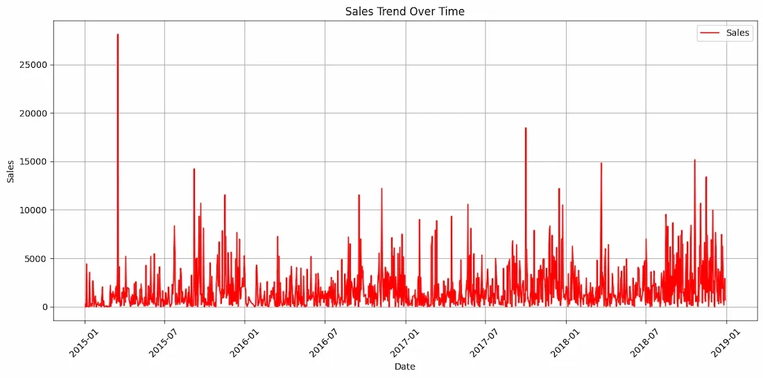 Sales Trend Over Time
4. Feature Engineering - Creating Lagged Features
Here we create lagged features to capture the temporal patterns in the sales data.
- create_lagged_features: This function generates lagged features by shifting the sales data by a given number of time steps like 1, 2, 3, etc. Lag features help the model learn from the previous sales data to predict future sales.
- dropna: Drops rows with missing values which are introduced due to the shift operation when lagging.
Python
def create_lagged_features(data, lag=1):
    lagged_data = data.copy()
    for i in range(1, lag+1):
        lagged_data[f'lag_{i}'] = lagged_data['Sales'].shift(i)
    return lagged_data

lag = 5
sales_with_lags = create_lagged_features(data[['Order Date', 'Sales']], lag)

sales_with_lags = sales_with_lags.dropna()
5. Preparing the Data for Training
In this step we prepare the data for training and testing.
- drop(columns): Removes the 'Order Date' and 'Sales' columns from the feature set
X since they are not needed for training as sales is the target variable. - train_test_split: Splits the dataset into training (80%) and testing (20%) sets.
shuffle=False: ensures that the data is split in chronological order preserving the time series structure.
Python
X = sales_with_lags.drop(columns=['Order Date', 'Sales'])
y = sales_with_lags['Sales']

X_train, X_test, y_train, y_test = train_test_split(X, y, test_size=0.2, shuffle=False)
6. Training the XGBoost Model
Here we will train the XGBoost model. It is a machine learning algorithm that uses gradient boosting to create highly accurate predictive models particularly well-suited for regression tasks like sales forecasting.
- XGBRegressor: Initializes an XGBoost model for regression tasks.
objective='reg:squarederror': indicates that we are solving a regression problem i.e predicting continuous sales values.- learning_rate (lr): Controls the step size at each iteration while moving toward a minimum of the loss function with smaller values leading to slower convergence.
- n_estimators: The number of boosting rounds or trees to build with higher values improving model accuracy but potentially leading to overfitting.
- max_depth: Defines the maximum depth of each decision tree controlling the complexity of the model. Deeper trees can model more complex patterns.
- fit: Trains the model on the training data (
X_train, y_train).
Python
model_xgb = xgb.XGBRegressor(objective='reg:squarederror', n_estimators=100, learning_rate=0.1, max_depth=5)
model_xgb.fit(X_train, y_train)
7. Making Predictions and Evaluating the Model
Here we make predictions and evaluate the model performance using RMSE.
- predict: Makes predictions on the test set (
X_test) using the trained XGBoost model. - mean_squared_error: Computes the Mean Squared Error (MSE) between actual and predicted values. We use
np.sqrt to compute the Root Mean Squared Error (RMSE), which is a standard metric for evaluating regression models.
Python
predictions_xgb = model_xgb.predict(X_test)
rmse_xgb = np.sqrt(mean_squared_error(y_test, predictions_xgb))

print(f"RMSE: {rmse_xgb:.2f}")
RMSE: 734.63
The RMSE of 734.63 indicates the average deviation between the actual and predicted sales values. A lower RMSE value signifies better model accuracy, with the model's predictions being closer to the actual sales data. As we have large amount of sales data this RMSE score is accptable.
8. Visualizing Results
We will plot both the actual and predicted sales to visually compare the performance of the model.
Python
plt.figure(figsize=(12, 6))
plt.plot(y_test.index, y_test, label='Actual Sales', color='red')
plt.plot(y_test.index, predictions_xgb, label='Predicted Sales', color='green')
plt.title('Sales Forecasting using XGBoost')
plt.xlabel('Date')
plt.ylabel('Sales')
plt.legend()
plt.grid(True)
plt.tight_layout()
plt.show()
Output:

As we can see the predicted and actual values are quite close to each other this proves the efficiency of our model. Sales forecasting using machine learning models like XGBoost can significantly enhance the accuracy of predictions by capturing temporal patterns in historical data. It can be used for improving sales predictions helping businesses optimize inventory, pricing and demand planning.
Similar Reads
Linear Regression for Single Prediction
Linear regression is a statistical method and machine learning foundation used to model relationship between a dependent variable and one or more independent variables. The primary goal is to predict the value of the dependent variable based on the values of the independent variables.Predicting a Si
6 min read
Forecast Function In R
The forecast function in R Programming Language is part of the forecast package, which provides functions and tools for forecasting time series data. This function allows users to generate forecasts for future time points based on historical data and time series models. The basic syntax of the forec
3 min read
Python | Pandas Series.product()
Pandas series is a One-dimensional ndarray with axis labels. The labels need not be unique but must be a hashable type. The object supports both integer- and label-based indexing and provides a host of methods for performing operations involving the index. Pandas Series.product() function returns th
3 min read
Steps of Forecasting
What is Forecasting?Forecasting is about making smart guesses about what might happen in the future by looking at past information and patterns using math-based methods. It's important for making choices, planning, and dealing with risks in areas, like business, money matters, economics, and even we
7 min read
Random Forest Regression in Python
A random forest is an ensemble learning method that combines the predictions from multiple decision trees to produce a more accurate and stable prediction. It is a type of supervised learning algorithm that can be used for both classification and regression tasks.In regression task we can use Random
9 min read
Python | Customer Churn Analysis Prediction
Customer Churn It is when an existing customer, user, subscriber, or any kind of return client stops doing business or ends the relationship with a company. Types of Customer Churn - Contractual Churn : When a customer is under a contract for a service and decides to cancel the service e.g. Cable TV
5 min read
Using SQLite Aggregate functions in Python
In this article, we are going to see how to use the aggregate function in SQLite Python. An aggregate function is a database management function that groups the values of numerous rows into a single summary value. Average (i.e., arithmetic mean), sum, max, min, Count are common aggregation functions
3 min read
Rainfall Prediction using Machine Learning - Python
Today there are no certain methods by using which we can predict whether there will be rainfall today or not. Even the meteorological department's prediction fails sometimes. In this article, we will learn how to build a machine-learning model which can predict whether there will be rainfall today o
6 min read
Python for Machine Learning
Welcome to "Python for Machine Learning," a comprehensive guide to mastering one of the most powerful tools in the data science toolkit. Python is widely recognized for its simplicity, versatility, and extensive ecosystem of libraries, making it the go-to programming language for machine learning. I
6 min read
Python | Pandas Period.quarter
Python is a great language for doing data analysis, primarily because of the fantastic ecosystem of data-centric python packages. Pandas is one of those packages and makes importing and analyzing data much easier. Pandas Period.quarter attribute return an integer value. The returned value represents
2 min read